Every chapter in this Part assumes the same upstream input: a stream of labelled outcomes. Backtests aggregate them. Brier scores assess their calibration. Monte Carlo bootstraps them. Walk-forward partitions them. The convergence card reports on them. The validation machinery is only as honest as the labels it consumes. Most retail systems label trades the laziest way possible: was the P&L positive or not? A win is a win, a loss is a loss, end of story. This is mathematically convenient and operationally catastrophic. It throws away the single most important piece of information about every closed trade: how the trade ended. The triple-barrier method, introduced by Marcos Lopez de Prado, fixes this by recording why each trade closed rather than just whether it made money.
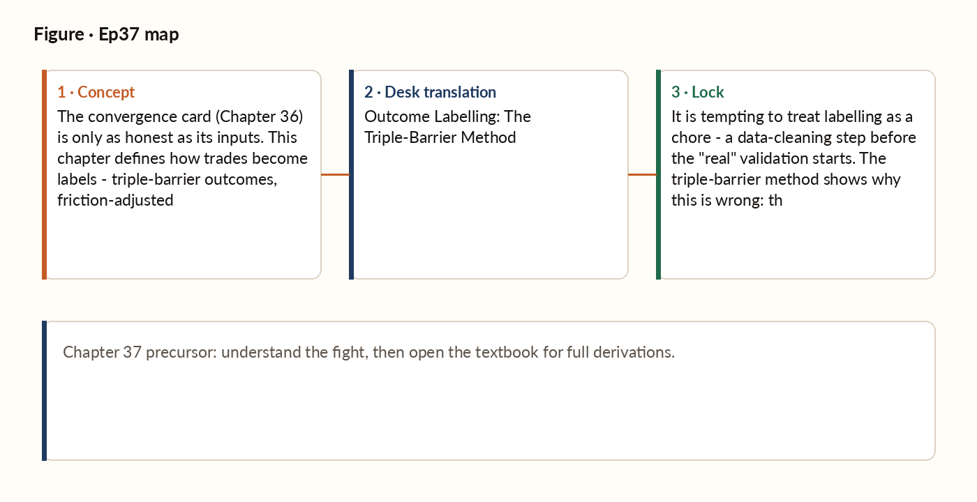
Figure 1. Concept map for this episode: fight, desk translation, what to lock.
The label pipeline — where triple-barrier sits
Triple-barrier is not a post-hoc report - it is the contract between execution and every downstream validator. The barrier widths are fixed when the trade is opened, execution records how the trade actually closed, and every downstream check - Brier scores, mean R, walk-forward, the convergence card - reads that same label rather than reconstructing its own story after the fact.
The three barriers
Every open trade has three exit triggers, called barriers. Upper barrier (take-profit, TP): a price level at which the trade is closed for a profit, typically set two volatility units (often measured via ATR, see Chapter 28) above entry. Lower barrier (stop-loss, SL): a price level at which the trade is closed for a loss, typically set one volatility unit below entry. Vertical barrier (time stop): a maximum holding period - commonly around ten trading days for a swing strategy - after which the trade is force-closed regardless of price. Whichever of the three the price path touches first decides the label.
What you can compute once you have barrier labels
The labels enable a family of conditional metrics that binary labels cannot: the fraction of trades that hit take-profit, hit stop-loss, or expired at the time stop. A high time-stop fraction means the setup is slow; a high stop-loss fraction means it is aggressive; a high take-profit fraction means it has real follow-through.
Setting the barrier widths
The three barrier settings are strategy-level hyperparameters chosen before the strategy runs, not optimised on each trade. Three standard choices: volatility-scaled, where the take-profit and stop-loss distances are set in units of recent realised volatility so a tight, low-vol bank stock gets narrower barriers than a volatile mining junior; risk-reward fixed, where the ratio between the two distances is held at a constant target (commonly 2:1) even as the absolute widths scale with volatility; and calendar-tuned time stops, where the holding-period limit is set to roughly the median time-to-resolution seen historically for similar setups, then revisited if too many trades start expiring at the limit. The Chapter 28 ATR machinery is the standard volatility unit.
Worked picture
Both strategies show 100 trades and mean R of 0.18 over a calibration window - identical on the surface. But look at how those trades actually closed. Strategy A: 36 take-profit hits, 54 stop-losses, 10 time-stops. Strategy B: 11 take-profit hits, 16 stop-losses, 73 time-stops. Strategy A's take-profit trades average +2.0R and its stop-losses -1.0R, exactly as designed, with its handful of time-stops averaging close to zero - a clean win rate of 36 in 46, about 78%. Strategy B's take-profit and stop-loss trades average the same +2.0R and -1.0R, but 73 of its 100 trades never really resolved - they just drifted to a small positive R of roughly +0.16 at the time stop, for a clean win rate of only 11 in 84, about 13%. Strategy A's mean R is earned: barely more than a third of its trades hit target outright, but they resolve cleanly and the 2:1 payoff on those clean wins carries the average. Strategy B's identical mean R is drift: 73% of its trades expire at the time stop, and the only reason the headline number looks respectable is that those time-stops average a small positive R purely by chance, not because the setup resolved in the strategy's favour. Strategy A deserves promotion; Strategy B should be investigated for an irrelevant setup that the holding-period mechanics happen to make weakly profitable. The improvement loop, fed binary labels, treats them identically. The improvement loop, fed triple-barrier labels, knows immediately which is which.
What breaks in production
The barriers MUST be set ex-ante, on theory or on a held-out sample. Tuning the take-profit distance, the stop-loss distance, or the time-stop length on the same trades whose labels you then use for validation is one of the cleanest examples of in-sample bias in the entire labelling pipeline. A particularly insidious version: "let me just nudge the time stop from 10 to 12 days, because then my time-stop rate drops by 5% and my hit rate looks better." This is exactly the kind of small, almost-invisible change that Chapter 32's warning about backtest sin was written for. Tuning the labels makes any downstream Brier score, p-value, or Sharpe ratio meaningless.
The labelling step is part of validation, not preprocessing
It is tempting to treat labelling as a chore - a data-cleaning step before the "real" validation starts. The triple-barrier method shows why this is wrong: the labels are validation. The choice of how to label a trade outcome determines what the downstream framework can see, and what it can see determines whether it can detect drift, mis-calibration, and creeping risk. A system that takes labelling seriously can run for years with stable validation metrics. A system that does not will eventually promote a drift-based strategy and be confused when it falls apart in production.