The motivating problem is brutally simple. A trader's swing position in a large-cap energy name loses 1.0R over a five-day holding window. The benchmark index fell 2% over the same window. Did the trade fail because the setup was wrong, or because the market fell and the name, being a high-β holding, fell with it? A naive validation machinery cannot tell. It charges the 1R loss to the strategy, the Brier score drifts upward, and the calibration loop dutifully nudges the scorecard's weights downward - even though nothing about the setup was actually wrong. Over weeks of choppy tape, this de-calibrates the model. The strategy was good; the market was just falling. The fix is CAPM β-attribution: split every trade's return into a market-driven piece and a setup-driven (idiosyncratic) piece, and only charge the setup-driven piece against the strategy's scorecard.
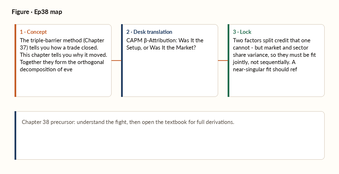
Figure 1. Concept map for this episode: fight, desk translation, what to lock.
Raw R vs idiosyncratic R — what the card charges
Not every metric should use the same return definition. Mixing them silently is how teams "fix" calibration by accident. When most of a strategy's recent closes turn out to be market-driven rather than setup-driven, the card should surface idiosyncratic mean R alongside raw mean R. A strategy can show positive idiosyncratic edge while the account bleeds in a down tape - the operator sizes via regime overlay (Part VII), not by rewriting the model after every macro week.
The CAPM decomposition
The Capital Asset Pricing Model (Sharpe 1964; Lintner 1965; Mossin 1966) is one of the foundational results in financial economics. In its simplest form, it asserts a linear relationship between a security's expected return and the market's expected return: a security's return is expected to move with the market in proportion to its beta - its sensitivity to market moves - plus whatever the risk-free rate contributes. For attribution purposes, what matters is the flip side of that relationship: any single trade's actual return can be split into a market-driven piece (beta times the market's move) and whatever is left over, the idiosyncratic piece the market cannot explain.
What "market" means
The choice of market index matters. For each security, the index should be: - Liquid: tradable, with continuous price data. - Broad: representative of the security's investable universe. - Same-currency: a USD security against a USD index; an INR security against an INR index. - Available with sufficient history: at least 252 trading days at the time of the beta estimation.
The attribution arithmetic on a single trade
Worked example. A trader closes a long position in a large-cap energy name with a return of -1.2% over a 5-day holding window. The benchmark index fell 1.8% over the same window. The name's rolling 252-day β against the index is 1.08 - meaning the name typically moves about 8% more than the index. So the market alone would have been expected to pull the position down by roughly 1.08 × 1.8% ≈ 1.94%. The position only fell 1.2%, which means the setup actually outperformed its market-implied counterfactual by about 0.74%. Charging the full 1.2% loss to the strategy would be misleading: the strategy beat expectations given how the market moved.
Definition
Extend the single-factor split with a second regressor: the return of a tradeable sector or industry proxy (an ETF or sector index). Now a trade's return splits three ways - a market beta, a sector beta, and whatever idiosyncratic residual is left. The market beta and the sector beta must be estimated jointly, not one after the other. Fitting the market beta alone and then fitting the sector beta on the leftover residual would silently assume the market and the sector are uncorrelated - they never are. A joint fit is the only way to split credit correctly between two overlapping explanators.
Worked picture
Same energy-name trade, same numbers as above. The improvement loop, fed the raw return: - Brier loss assigned to the strategy: roughly 0.04 (depending on the predicted probability). - Strategy's rolling Brier ticks upward. - After many such "losses," the scorecard's weights drift downward. The improvement loop, fed the idiosyncratic return: - The trade is counted as an idiosyncratic win (with the market component logged separately for the regime-overlay's diagnostics). - Brier loss assigned to the strategy: near zero (the strategy correctly predicted positive idiosyncratic return). - The scorecard's weights stay stable. The market component does not disappear - it shows up on the regime overlay's scorecard, where it belongs. Bad regime calls cost the regime overlay; bad setup calls cost the setup model. Attribution gives each subsystem its own honest report card.
What breaks in production
Pairing a small-cap semiconductor name against a large-cap-dominated benchmark index will produce a misleadingly small β - the small-cap moves on different forces. The "idiosyncratic" residual then absorbs much of the small-cap-as-an-asset-class signal, defeating the purpose of attribution. The defence: match the index to the security's investable universe as closely as feasible. When in doubt, run the attribution with two indices and compare - large discrepancies are evidence the chosen index is wrong.
Key idea
Two factors split credit that one cannot - but market and sector share variance, so they must be fit jointly, not sequentially. A near-singular fit should refuse to report a split rather than report an unstable one: an honest "unavailable" beats a confident, meaningless number.