The Monte Carlo simulations of Chapter 33 require a model of the per-trade distribution. The bootstrap is a non-parametric alternative that simulates by resampling the actual historical observations - assuming nothing about the underlying distribution beyond the assumption that the historical sample is representative. This is one of the most important developments in 20th-century statistics. Before the bootstrap, computing a standard error for a statistic like the median, the Sharpe ratio, or the maximum drawdown required either parametric assumptions (which are often wrong) or large-sample approximations (which are often inaccurate for the small samples we have in trading). The bootstrap, proposed by Bradley Efron in 1979, sidesteps both.
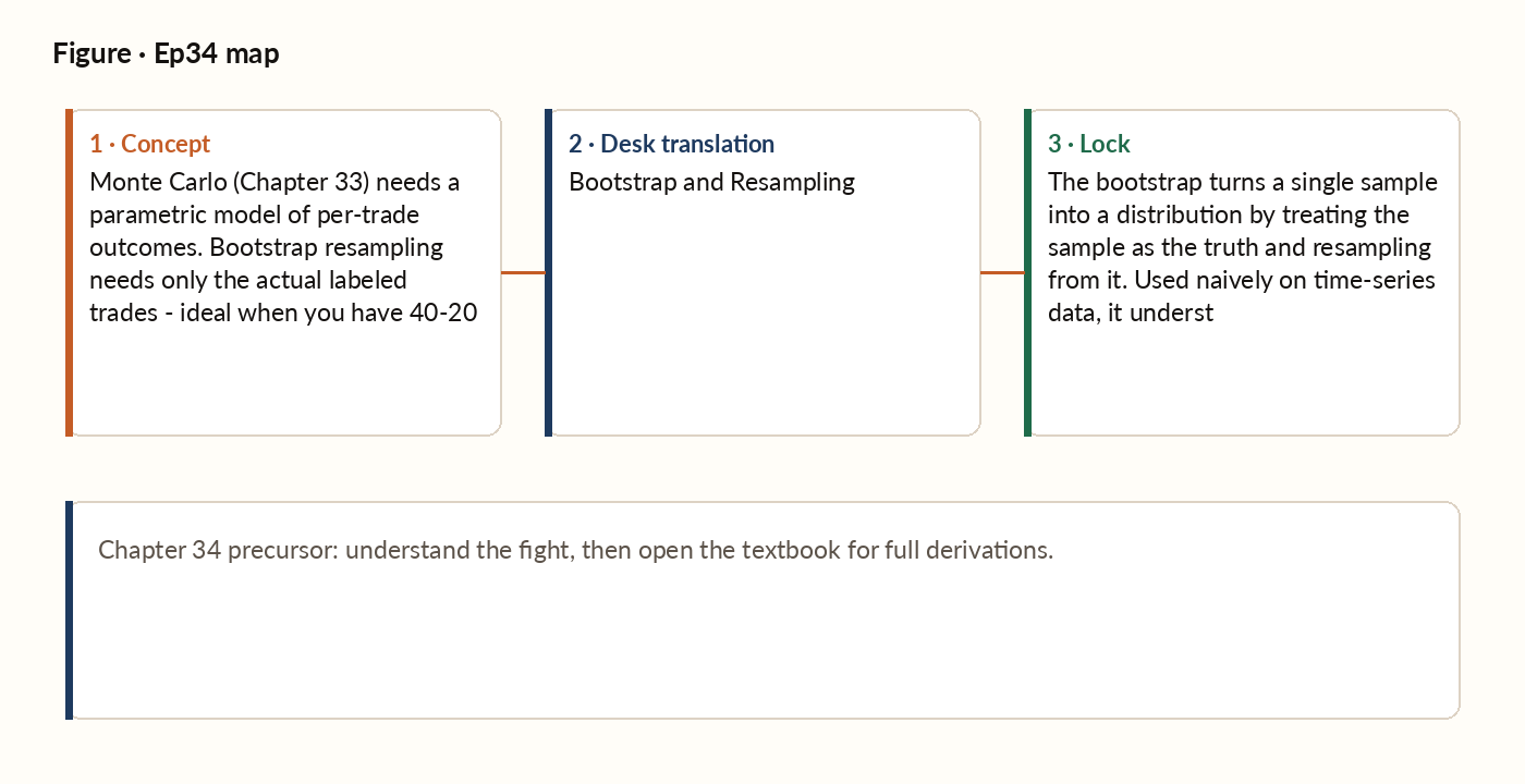
Figure 1. Concept map for this episode: fight, desk translation, what to lock.
The bootstrap procedure
Given a sample of observations, the bootstrap procedure is: sample observations with replacement from the original sample - each draw selects one of the original observations at random, and the same observation can be picked more than once. Call this a bootstrap sample. Compute the statistic of interest (mean, Sharpe, drawdown, whatever you care about) on that sample. Repeat this thousands of times, and the spread of results approximates how uncertain your original estimate really is.
Confidence intervals from the bootstrap
The most common use of the bootstrap is to construct confidence intervals. After thousands of bootstrap estimates, a 95% confidence interval for the true value is simply the middle 95% of those estimates - the 2.5th percentile up to the 97.5th percentile of the bootstrap distribution. This is the percentile bootstrap. More sophisticated variants - BCa (bias-corrected and accelerated), studentized bootstrap - refine the estimate but are usually unnecessary for trading applications.
The block bootstrap for time series
The naive bootstrap of §34.1 assumes independence of observations. For time-series data, this assumption is wrong - today's return is correlated with yesterday's; today's volatility is correlated with yesterday's. The naive bootstrap therefore understates the true uncertainty, producing confidence intervals that are too narrow. The block bootstrap resamples contiguous blocks of observations rather than individual observations - preserving the local autocorrelation within each block while still breaking up long-range dependence across blocks, so the resulting confidence intervals correctly account for the serial correlation in the original data.
Practical applications
A key trading application of the bootstrap: Sharpe ratio confidence intervals. Compute the Sharpe of each bootstrap sample. The 5th-95th percentile range is the 90% CI for the true Sharpe. A Sharpe whose CI includes zero is not statistically distinguishable from a null strategy - no matter how good the point estimate looks. The same trick works for maximum drawdown (bootstrap the equity curve and take the 95th percentile of drawdowns as a robust worst-case estimate) and for feature significance (bootstrap the period-by-period IC observations from Chapter 13 and check whether the resulting distribution of mean ICs includes zero).
Worked picture
You have 250 daily returns from a strategy. The realised Sharpe is 1.4. What is the 95% CI? Procedure: draw 10,000 bootstrap samples (each of 250 daily returns sampled with replacement from the original 250). For each sample, compute the Sharpe. Sort the 10,000 Sharpes. The 250th and 9,750th are your 2.5th and 97.5th percentiles. Suppose the 2.5th percentile is 0.6 and the 97.5th is 2.2. The 95% CI is (0.6, 2.2). The CI is wide because 250 daily observations is a modest sample; the realised Sharpe of 1.4 is consistent with a true Sharpe anywhere from 0.6 to 2.2. The CI includes values both below 0.5 (probably not worth running) and above 2.0 (genuinely excellent). A capital allocator should treat the strategy with appropriate humility: the realised 1.4 is your best point estimate, but the true Sharpe could plausibly be much lower. More data is the only fix.
What breaks in production
A common mistake: take 1,000 days of strategy returns, bootstrap individual days, and report a bootstrap CI for the Sharpe ratio that is half the width of the true CI. The strategy looks more reliable than it is. Subsequent live performance is more variable than the bootstrap suggested. The capital allocator who relied on the narrow CI sized too aggressively and got hurt. Always check the autocorrelation of your data series before using the bootstrap. If the lag-1 autocorrelation is greater than 0.1, switch to the block bootstrap. If you do not know how to compute the autocorrelation, use the block bootstrap anyway - it costs nothing extra and protects against an easy mistake.
Key idea
The bootstrap turns a single sample into a distribution by treating the sample as the truth and resampling from it. Used naively on time-series data, it understates uncertainty; the block bootstrap is the correct tool. Reports of single-number Sharpes, drawdowns, or returns without confidence intervals should be treated as preliminary and incomplete.