Given a feature vector for the current candidate trade, KNN works as follows: find the historical observations whose feature vectors are most similar to the current one, by some distance metric; look at the realised outcomes (wins/losses, or returns) of those similar observations; then predict the current trade's outcome as the average of those neighbours' outcomes.
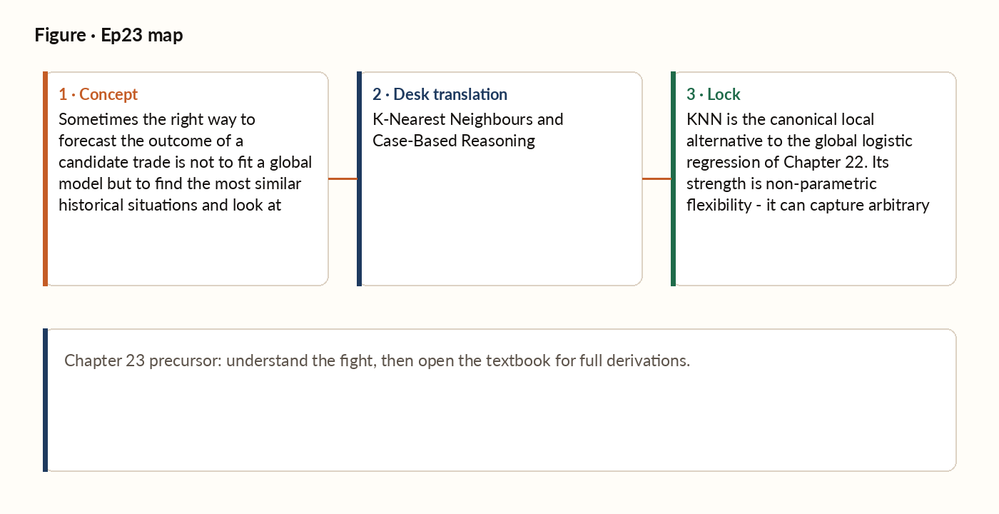
Figure 1. Concept map for this episode: fight, desk translation, what to lock.
The distance metric
The most common distance metric is Euclidean distance: the straight-line distance between two feature vectors, computed the same way you'd measure distance on a map. Important: the features must be on comparable scales, or the distance is dominated by whichever feature has the largest scale. The standard fix is to standardise all features (zero mean, unit variance) before computing distance.
Application to trading: the historical analogue
In trading, KNN is often used as a historical analogue layer. Given a current setup's features, find the 20 or so most similar historical setups and report the empirical win rate (and return distribution) of those neighbours. This produces a non-parametric probability estimate that does not assume a particular functional form. It also produces a natural sanity check: if the 20 nearest historical analogues have an empirical win rate of 0.65, the candidate trade has stronger evidence than if the same setup had only 2 historical neighbours and a 0.50 win rate.
Worked example
Suppose the current candidate has some standardised feature vector. You search the historical database and find the 5 nearest historical setups, and 4 of the 5 turned out to be wins. Empirical win rate among the 5 neighbours: 4/5 = 0.80. The historical-analogue forecast is a win probability of about 0.80, with a wide confidence interval since 5 examples is a small sample.
What breaks in production
In low-dimensional space (say, 3 features), distances are meaningful. The 10 nearest neighbours of any query point are genuinely "similar" along the feature dimensions. In high-dimensional space (say, 50 features), distances become uninformative. Almost all points are roughly equidistant from any query point - a counterintuitive consequence of geometry in high dimensions. The "10 nearest neighbours" of a query include points that are not actually similar in any meaningful sense; they just happen to win the lottery of distance computation noise. The fix is dimensionality reduction before KNN: PCA, autoencoders, or learned embeddings (Chapter 24) compress the feature space into 10-20 dimensions where distances are still meaningful. KNN on raw 50-dimensional structured features rarely works well; KNN on a 16-dimensional embedding of the same data typically does. The rule of thumb: KNN works in dimensions below 20 or so. Above that, embed first.
The other production problem: search speed
Dimensionality is not the only thing that breaks. For a historical database of N observations, naive nearest-neighbour search costs O(N) per query — fine for a few thousand rows, unworkable once the case-book grows into the millions. The standard fix is approximate nearest-neighbour search using data structures like KD-trees, ball trees, or locality-sensitive hashing: production vector indexes return approximate neighbours in microseconds even against billions of stored cases. The word "approximate" rarely costs anything in practice here — the difference between the true 20 nearest neighbours and an approximation that finds 19 of them is operationally negligible for a sizing decision that is already averaging over a handful of noisy historical outcomes.
Key idea
KNN is the canonical local alternative to the global logistic regression of Chapter 22. Its strength is non-parametric flexibility - it can capture arbitrary structure without assuming a functional form. Its weaknesses are the curse of dimensionality and the data-structure cost of search at scale. In practice, KNN is most often used as a historical-analogue augmentation to a global scorecard, providing sanity checks and confidence-interval information rather than driving sizing decisions on its own.