Here IR is the Information Ratio (the active return per unit of active risk), IC is the Information Coefficient (the cross-sectional correlation of forecast with realised return), and breadth is the number of independent bets per period. The relationship is one of the most-cited and most-misunderstood results in finance. This chapter derives it, dissects its assumptions, and connects it to the breadth/effective-N analysis in Chapter 18.
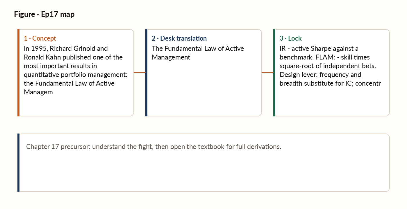
Figure 1. Concept map for this episode: fight, desk translation, what to lock.
What "active" means
An active strategy is one whose returns are measured relative to a benchmark. The active return of a portfolio in a given period is simply its return minus the benchmark's return over that same period. The active risk is the standard deviation of that active return over time - how much the portfolio's edge over the benchmark actually wobbles.
The derivation of FLAM
The result follows from a few reasonable assumptions: the portfolio takes active positions proportional to its forecast signals; those forecasts have some real correlation with realised returns (the IC from Chapter 13); the universe of investable assets is reasonably large; and, crucially, the assets are assumed to be uncorrelated with each other cross-sectionally - an assumption Chapter 18 attacks in detail. Under these assumptions, the diversification benefit from spreading bets across many assets and many periods compounds in a specific way: the Information Ratio scales with skill (IC) times the square root of the total number of independent bets you make, across both names and time.
Implications for trading strategy design
FLAM has dramatic consequences for how strategies should be designed. A small IC scales beautifully with breadth. A modest 0.02 IC deployed across 500 names and 250 trading days a year delivers a phenomenal Information Ratio above 7 - if the bets are truly independent. (They are not, which is the whole point of Chapter 18.)
The catch: independence
The derivation assumes the bets per period are independent. They almost never are in practice. Two stocks in the same sector are correlated; two factor portfolios with overlapping holdings are correlated; two momentum signals with similar lookback windows are correlated. When bets are correlated, the effective breadth is less than the nominal count. We will develop the precise formula in Chapter 18, but the intuition is simple: if your 200 active positions are really only 50 effective bets (the rest being correlated duplicates), your true Information Ratio is a full 2x lower than the naive count would suggest.
Worked picture
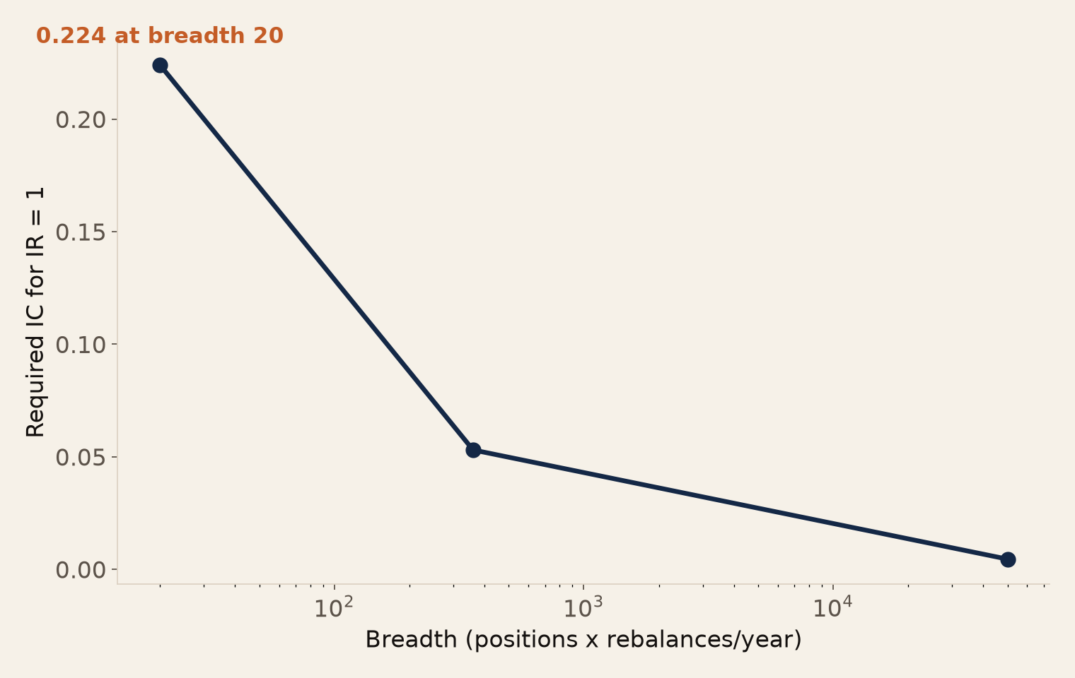
A long-short equity scanner running 200 simultaneous positions, rebalanced 250 times a year, has around 50,000 independent bets - so the IC needed to hit an Information Ratio of 1.0 is tiny, well under 1%. A monthly factor portfolio with 30 positions rebalanced 12 times a year has only about 360 bets, so it needs a more modest but still achievable IC of around 5%. A quarterly concentrated stock-picking book with just 5 positions, rebalanced 4 times a year, has only about 20 bets - and needs an IC north of 20% to hit the same target, a level of forecasting skill essentially no one achieves. The lesson: strategy design choices about breadth and frequency are at least as important as forecasting skill. A great forecaster constrained to a low-breadth strategy will have mediocre IR; a mediocre forecaster with a high-breadth strategy will have excellent IR.
Figure. Required IC to hit IR=1 falls sharply as breadth rises — 0.224 at breadth 20 down to 0.0045 at breadth 50,000.
What breaks in production
A trader runs a long-short portfolio with 100 longs and 100 shorts - 200 active positions in total. Naive FLAM says BR = 200 per rebalance. In reality, the 100 longs might be 100 momentum names with 70% pairwise correlation (they all rise together in a momentum regime, fall together in mean reversion). The effective independent positions might be 5-10. Same for the shorts. The realistic breadth is closer to 20 - a factor-of-ten gap between nominal and effective breadth. The expected IR is correspondingly about 3.2x lower than the naive FLAM calculation suggests. If you sized the strategy assuming a breadth of 200, you have effectively over-sized by a factor of 3.2. The realised Sharpe will be 1/3.2 = 0.3x your expectation - and you will be confused about why.
Chapter 17 — the picture closes
IR is active Sharpe against a benchmark. FLAM says it's skill times the square root of independent bets. Design lever: frequency and breadth substitute for IC; concentrated books need impossible IC. Ceiling check: backtest IR above the FLAM ceiling implies overfit until proven otherwise. IC from Chapter 13 was always a per-bet whisper; FLAM is how loud it gets across the book.