Effective N: Why Three Signals Are Not Three Signals

Suppose you have a set of signals with some pairwise correlation between them. The effective N is a single number that tells you how many genuinely independent signals your correlated set is really worth - it will always be less than or equal to the number of signals you actually have, and it shrinks the more those signals overlap with each other.

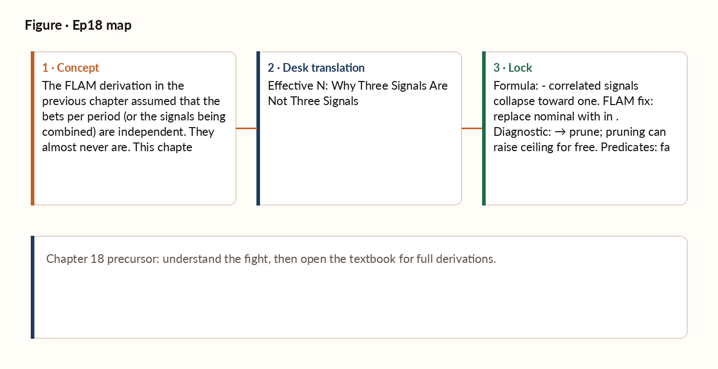
Figure 1. Concept map for this episode: fight, desk translation, what to lock.

The effective-N formula

Suppose you have a set of signals with some average pairwise correlation between them. The effective N shrinks smoothly as that average correlation rises: with zero correlation, effective N equals the full signal count; as correlation climbs toward perfect (every signal a clone of every other), effective N collapses toward just one.

The two extremes

The effective-N formula has two illuminating limits. At one extreme, independence: if all off-diagonal correlations are zero, the effective N equals the actual signal count. Each additional signal is genuinely independent, and breadth grows linearly with the number of signals. At the other extreme, perfect correlation: if every signal is a clone of every other, the effective N is 1 no matter how many signals you have - adding more is pure noise, because they all move together. A realistic panel of, say, 10 signals with an average correlation of 0.2 works out to an effective N of about 3.6: ten signals collapse into roughly 3.6 effective ones.

The FLAM correction

The naive FLAM calculation uses the nominal signal count; the corrected version uses the effective N instead. For that same example (10 signals, effective N of 3.6), the naive FLAM overstates the Information Ratio by a factor of about 1.67 - a backtest IR of 2.0 should be revised down to about 1.2 once the correlation among signals is properly accounted for.

The redundancy diagnostic

The effective-N formula gives a diagnostic for whether a panel of features is well-constructed or full of duplicates. When effective N sits close to the nominal count, features are essentially independent - the panel is well-designed and each feature contributes incremental information. As that ratio drops below roughly 0.3, features are moderately to heavily redundant, and pruning becomes worthwhile; below 0.1, the panel is essentially duplicates and needs aggressive deprecation.

Worked picture

The 14-feature panel

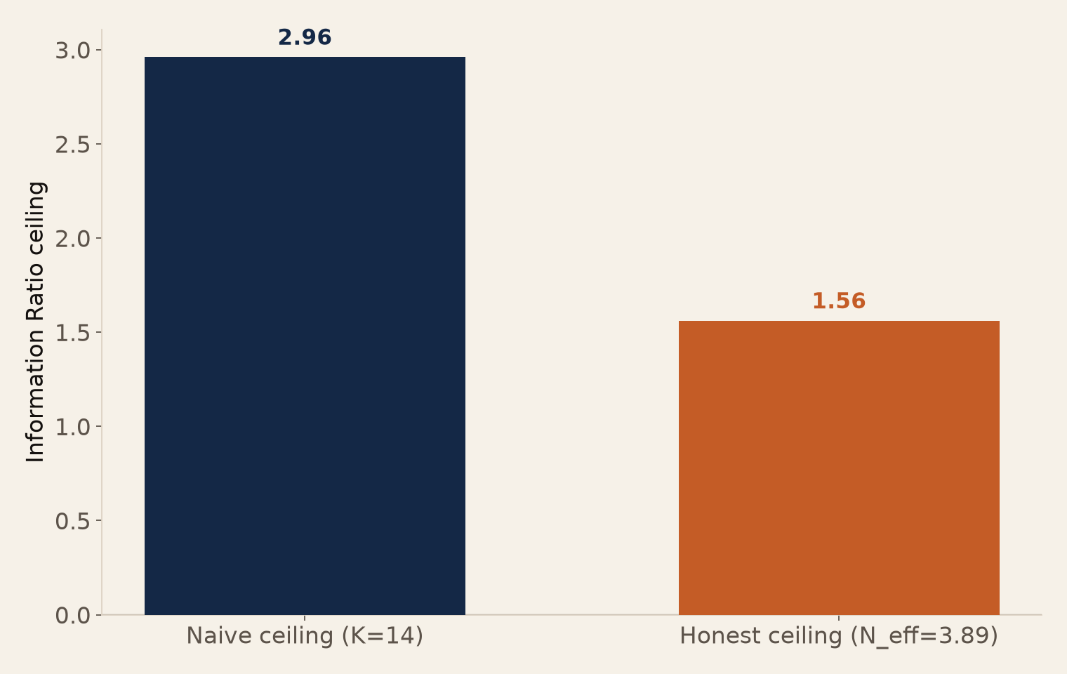
A trading scorecard uses 14 features. The correlation matrix has off-diagonal entries averaging 0.20. Some pairs are higher (two "momentum" features at 0.6 correlation); some are lower (a fundamental feature against a microstructure feature at 0.05). Working through the formula, the effective N comes out to about 3.89. The panel claims to use 14 features but is effectively 3.89 independent features. The FLAM-implied IR ceiling is therefore built on that smaller number, not the nominal 14. For a year of daily rebalancing and an IC of 0.05, the honest ceiling comes out to about 1.56, versus a naive (and wrong) estimate of 2.96 if you'd used the full 14.

Figure. The naive IR ceiling (treating 14 correlated features as independent) vs. the honest ceiling once N_eff=3.89 replaces the raw count.

The strategy can achieve at most that lower IR in production, no matter how well-tuned the weights. Any backtest claiming materially higher IR is overfit, and the most likely culprits are (a) implicit over-fitting of the weight vector to historical correlations, or (b) the in-sample correlations being lower than the out-of-sample correlations.

Predicates: the same diagnostic at a different scale

Everything above applies directly to a continuous feature panel, but the same correlation logic also governs the boolean "if-then" rules a predicate miner generates from that panel - thousands of candidates like "momentum above this threshold and news score above that one." The underlying features might have low correlation, but two thresholds carved from the same feature are nearly duplicates of each other: a rule that fires on "feature above 0.3" and one that fires on "feature above 0.4" will co-trigger on most of the same rows. The fix is to group predicates that share a parent feature into a family, Bonferroni-correct within each family using that family's own (small) size, then aggregate across families using something close to the effective number of families rather than the enormous nominal candidate count. A family of 8 threshold-rules on one feature, correlated at about 0.85 with each other, behaves like roughly 1.2 effective rules - eight variations on one idea, not eight independent discoveries. On top of the two Bonferroni layers, apply a support floor at the individual-predicate level: a rule that fires on only a handful of rows out of a corpus of thousands is technically present but statistically silent, and gets rejected regardless of how good its in-sample win rate looks.