When observations are positively autocorrelated, the naive standard error of the sample mean underestimates the true uncertainty. The t-statistics computed with the naive standard error are too large. Hypotheses are rejected too often. False positives flood the research pipeline. The fix is the Newey-West HAC standard error - Heteroskedasticity and Autocorrelation Consistent - developed by Whitney Newey and Kenneth West in 1987. It is the workhorse correction for time-series statistics in quantitative finance.
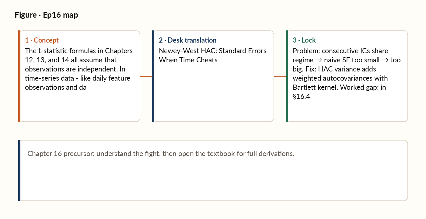
Figure 1. Concept map for this episode: fight, desk translation, what to lock.
The autocorrelation problem
Suppose you observe a daily time series of some statistic. The naive estimate of the variance of the sample mean simply divides the sample variance by the number of observations - a formula that assumes each day's observation is unrelated to the last. If consecutive days are positively correlated instead, that assumption breaks: with a fairly typical daily autocorrelation of 0.3, the true variance of the sample mean runs about 1.6 times higher than the naive formula suggests, meaning the true standard error is about 26% higher than the naive one. A feature whose naive t-statistic reads 2.5 is really closer to 2.0 once you correct for this - much closer to the edge of insignificance.
The Newey-West formula
The Newey-West HAC variance estimator generalises the naive formula to handle arbitrary autocorrelation structures. Rather than just dividing the variance by the sample size, it adds in the covariances between each observation and its recent neighbors, with more distant lags counted less and less (a "Bartlett" weighting scheme) so the correction fades out smoothly rather than cutting off abruptly.
Choosing the lag length L
The Newey-West formula requires choosing how many lags of that fading correction to include. The standard rule of thumb (Andrews' rule) scales gently with the sample size: for 100 daily observations you'd typically use about 4 lags, for 250 observations about 5, and for 1,000 observations about 7. In trading applications, a lag count between 3 and 10 is typical - larger for highly autocorrelated series like macro features, smaller for series that are nearly independent day to day.
Worked example: correcting a feature's t-statistic
Suppose you compute daily ICs for a feature over 100 days. The mean IC is 0.045 and the sample standard deviation is 0.060. The naive standard error is 0.006, giving a naive t-statistic of 7.5 - looks dramatically significant. But you compute the first-order autocorrelation of the IC series and find it to be 0.30. Applying the Newey-West correction with 4 lags and Bartlett weights, the corrected t-statistic comes out to 5.84 - still comfortably above the significance threshold, but a meaningfully more honest number than the naive 7.5.
Worked picture
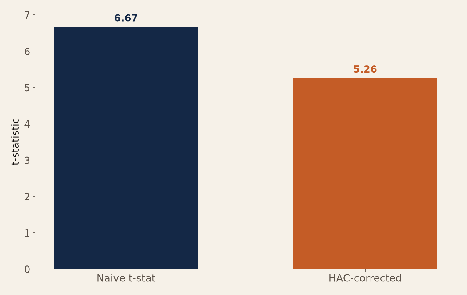
Daily IC series: mean IC 0.04, sample SD 0.06, 100 days, lag-1 autocorrelation 0.30. Naive SE works out to 0.006 → naive t of 6.67 - looks bulletproof. The first-order inflation factor (about 1.26x for this autocorrelation) pushes the adjusted SE up to about 0.0076 → adjusted t of about 5.26. Still significant, but 21% of the apparent strength was shared weather between consecutive days. At a borderline t near 2.2, this correction flips the verdict - time cheats before Bonferroni even opens the file.
Figure. Naive vs. HAC-corrected t-statistic — for IC mean 0.04, autocorrelation 0.30, naive t=6.67 drops to 5.26 once dependence is corrected.
What breaks in production
A research project that involves look-ahead bias, survivorship bias, or in-sample tuning cannot be saved by Newey-West HAC. HAC corrects for one specific bias - the inflated t-statistic from autocorrelated observations - and assumes all other assumptions hold. If you apply HAC to a study that has a fundamental design flaw, you get a more accurate p-value for a fundamentally flawed hypothesis. The flawed conclusion remains flawed. HAC is a correction, not a cure.
Chapter 16 — the picture closes
Problem: consecutive ICs share regime → naive standard error too small → t-statistic too big. Fix: HAC variance adds weighted autocovariances with a Bartlett kernel. Worked gap: t fell from 7.5 to 5.84 in the worked example above - still significant, but not miraculous. Limit: HAC fixes dependence, not look-ahead bias, survivorship bias, or how many features you tested. Correct the time series first; Bonferroni the panel second; only then size (Part II).