Suppose you are testing a number of hypotheses, each at the usual significance level (typically 0.05). The Bonferroni correction tells you to use a much stricter per-test significance level: split the usual 5% evenly across every test you run, so each individual test has to clear a tougher bar. Test 10 hypotheses and the per-test bar drops to 0.005. Test 100, and it drops to 0.0005. Test 1,000, and it drops to 0.00005.
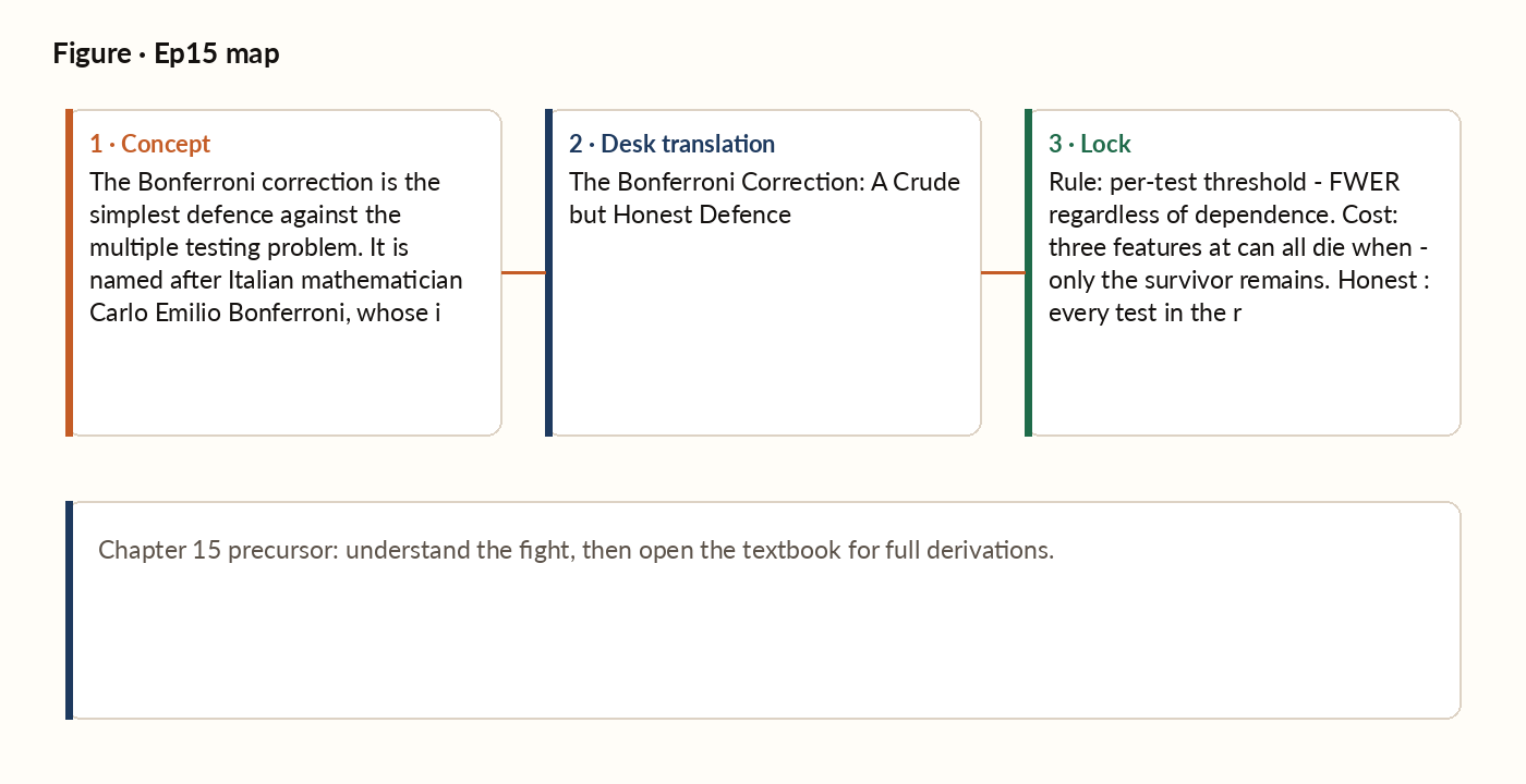
Figure 1. Concept map for this episode: fight, desk translation, what to lock.
The procedure
Suppose you are testing a number of hypotheses, each at the usual significance level (typically 0.05). The Bonferroni correction tells you to use a much stricter per-test significance level: split the usual 5% evenly across every test you run, so each individual test has to clear a tougher bar. Test 10 hypotheses and the per-test bar drops to 0.005. Test 100, and it drops to 0.0005. Test 1,000, and it drops to 0.00005. This is all there is to Bonferroni. The threshold gets stricter as you test more hypotheses. The arithmetic is trivial.
The conservativeness of Bonferroni
The Bonferroni inequality becomes an equality only when the events are mutually exclusive - when no two false positives can occur simultaneously. In practice, when features are correlated, false positives tend to come in groups (correlated features fail together), and Bonferroni overcorrects. How much does Bonferroni overcorrect? For perfectly independent tests, the actual false-positive rate under no correction is very close to what Bonferroni assumes - so Bonferroni is nearly exact for independent tests. For correlated tests, the true false-positive rate without correction is lower than Bonferroni assumes (because correlated failures bunch together instead of spreading out), so Bonferroni ends up overly cautious.
Worked example
Suppose you test 20 candidate features and get back their t-statistics. At the uncorrected 5% threshold, four features - call them F1, F2, F3, and F4 - all clear the bar. Naively, you would declare them all significant. But applying the Bonferroni correction for 20 tests drops the bar to 0.0025, and only the strongest of the four (with a p-value of 0.0002) still clears it. The other three are rejected as plausibly noise once you account for how many tests you ran.
Beyond Bonferroni: Holm-Sidak and FDR
For applications where Bonferroni is too conservative, two refinements are common. Holm-Sidak is a sequential variant. Sort your results from most to least significant, then test each one against a progressively looser bar as you work down the list. This is strictly more powerful than Bonferroni (rejects at least as many hypotheses) and still controls the family-wise error rate.
Worked picture
Suppose your trading system has a panel of 20 features, of which 14 are "live" (used in scoring) and 6 are deprecated. You run a feature-significance diagnostic on the live panel, computing the Pearson IC and Newey-West-corrected t-statistic for each feature against next-week returns over the last 90 days. Three features have raw p-values below 0.05: Feature A (gap-up reversal) at 0.018, Feature B (volume spike) at 0.032, and Feature C (catalyst flag) at 0.047. But the Bonferroni-corrected threshold for 14 tests is roughly 0.0036, and none of the three clear it. The interpretation: with the data you have (90 days), none of the features has demonstrated statistically significant predictive content after accounting for the fact that you tested 14 features. This does not mean the features are useless. It means the evidence is not yet strong enough to make a high-confidence statement. The features may still be in the live panel - operational use is a different question from statistical significance - but the recent diagnostic does not justify increasing their weight. The fix is more data: with four times as much history, the standard errors shrink and the t-statistics roughly double, so features with a genuine edge will eventually clear the bar.
What breaks in production
The single biggest practical error in applying Bonferroni is undercounting how many tests you've actually run. The honest count includes every test you ever ran on this data - not just the tests you decided to report. If you tested 50 features over the last year and are now testing one more, the count for the new feature is 51, not 1. In serious quant shops, this is enforced by a research registry - every test run on the dataset is logged with timestamp, hypothesis, and outcome. The count for any new test is the size of the registry to date. This sounds paranoid but it is the only way to keep the multiple-testing correction honest over multi-year research programmes.
Chapter 15 — the picture closes
Rule: split the significance threshold evenly across every test you run, and the overall false-positive rate stays controlled no matter how the tests are related. Cost: three features that each looked individually significant can all die once you correct for testing 20 of them - only the strongest survivor remains. Honest count: every test in the registry counts, not just the ones in the slide deck. Pair with HAC: fix the standard errors for autocorrelation first (Chapter 16), then apply Bonferroni. Crude, conservative, and exactly the receipt the multiple-testing detective asked for.