The Brier Score and Murphy Decomposition

For a sequence of probabilistic forecasts matched against what actually happened, the Brier score is the average squared error between each forecast probability and the realised outcome (scored as 1 for a win, 0 for a loss). A perfect forecaster who always predicts 1 when the outcome is 1 and 0 when the outcome is 0 has a Brier score of 0. A forecaster who always predicts 0.5 regardless of outcome has a Brier score of 0.25 (the variance of a fair coin). A worse-than-random forecaster has a Brier score above 0.25.

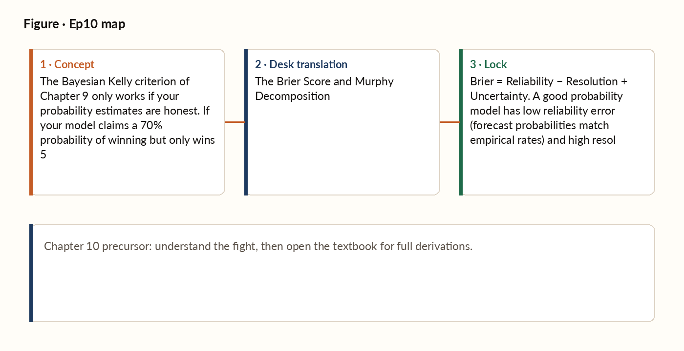
Figure 1. Concept map for this episode: fight, desk translation, what to lock.

The Brier score formula

Squared error is used here, rather than plain absolute error, because it uniquely rewards a forecaster for reporting their true believed probability. A forecaster who believes a 60% chance but rounds up to 70% "to sound confident" ends up with a worse expected score than if they had just reported 60% honestly. Absolute-error scoring doesn't have this property. It actually rewards forecasters for rounding toward 0% or 100%, which is exactly the dishonest behaviour we want to discourage.

Decomposing the Brier score

The single Brier number conceals what is actually going on. Statistician Allan Murphy showed in 1973 that the Brier score decomposes into three meaningful components, each isolating a different way a probability forecast can be wrong. To compute the decomposition, bin the forecasts into groups by predicted probability. Say, predictions near 0.1 go into one bin, predictions near 0.2 into the next, and so on. Then compare, within each bin, the average forecast to the actual empirical outcome rate. The three components are: reliability (how far the forecasts are from the empirical rates within each bin; smaller is better), resolution (how much the bins differ from each other; larger is better, since it means the model is actually discriminating), and uncertainty (a fixed baseline set entirely by the base rate of the data, which no amount of modelling skill can improve on).

What each component tells you to fix

The Murphy decomposition is operationally useful because each component points to a specific type of model defect. High reliability error means your model is mis-calibrated. It is saying 0.7 when it should be saying 0.5, or vice versa. The fix is recalibration. Train an isotonic or Platt-scaling layer on top of your model's raw outputs: a small secondary fit (a monotonic step function for isotonic regression, a logistic curve for Platt scaling) that stretches or compresses your raw probability scale to match empirical frequencies, without changing which trades rank above which. This is a post-hoc fix that doesn't require retraining the underlying model. Low resolution means your model is uninformative, producing outputs near the base rate regardless of input; the fix here is better features or more data, since recalibration alone can't create discrimination that isn't there. High uncertainty relative to your peers means the underlying problem itself is just hard, and there's a hard floor on how good any forecast can get.

Calibration plots: visualising reliability

A standard way to visualise the reliability component is the calibration plot (also called a reliability diagram). On the horizontal axis, plot the predicted probability for each bin. On the vertical axis, plot the empirical outcome rate for that bin. Add a 45-degree line as the ideal.

Figure. A real reliability diagram: four calibration bins from a Brier-0.21 worked example (n=400), plotted predicted vs. empirical — all four sit close to the diagonal.

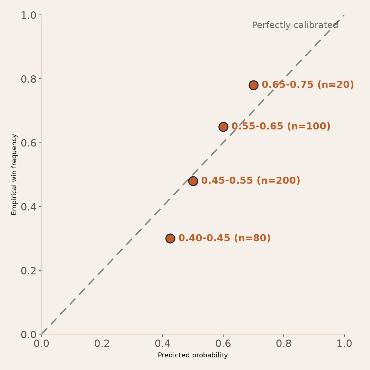
A perfectly calibrated model lies exactly on the 45-degree line. A model that is systematically over-confident sits above the diagonal in the high-probability bins (saying 0.8 but only winning 0.6 of the time). A model that is systematically under-confident sits below the diagonal instead.

Worked picture