The Bayesian Kelly criterion (sometimes called the posterior-weighted Kelly) formalises this shrinkage. It combines the Bayesian posterior from Chapter 7 with the Kelly formula from Chapter 8 to produce a bet size that is both growth-optimal and robust to estimation error. Suppose you observe 6 wins in 10 trades. The empirical win rate is 60%, suggesting a naive Kelly bet of 20% of capital. But after only 10 trades, that estimate is extremely uncertain: the true win rate could plausibly be anywhere from about 29% to 91%. If the truth is actually 30% (a losing edge!), the correct Kelly bet is negative. You should be short the strategy, not long it. If the truth is 91%, an 82% Kelly bet would have been correct instead. The naive estimate hides all of this.
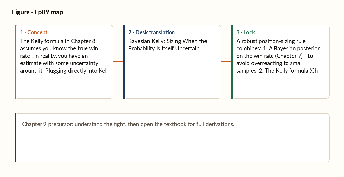
Figure 1. Concept map for this episode: fight, desk translation, what to lock.
The problem with naive Kelly
Suppose you observe 6 wins in 10 trades. The empirical win rate is 60%, suggesting a naive Kelly bet of 20%. But after only 10 trades, that estimate carries a huge amount of uncertainty. Wide enough that the true win rate could plausibly sit anywhere from about 29% to 91%. At the low end of that range you have a losing edge and should be short, not long; at the high end, a much larger bet than 20% would be justified. The naive plug-in estimate ignores all this. It treats the empirical 60% as the truth and bets accordingly. With high probability you are betting too much. The expected cost of over-betting is much larger than the expected gain from under-betting, because the Kelly growth curve is asymmetric around its peak. It falls off a cliff on the aggressive side and only tapers gently on the conservative side.
The Bayesian Kelly fraction
The correct Bayesian approach is to weigh the Kelly formula across the whole posterior distribution of the win rate, rather than plugging in a single point estimate. For an even-money bet, this works out to a clean result: the Bayesian Kelly fraction is exactly the ordinary Kelly formula, but computed using the posterior mean instead of the raw empirical win rate. In other words: do not size on the empirical mean, size on the Bayesian posterior mean. The posterior mean already shrinks toward the prior, which automatically protects you from over-betting on small-sample noise.
Adding a variance shrinkage
The posterior-mean Kelly above already shrinks the point estimate toward the prior. But for very small samples, the posterior itself is still wide, and we want to penalise that remaining uncertainty further. The clean way to derive the appropriate shrinkage is a second-order Taylor expansion of expected log-growth around the optimal bet fraction. This produces an extra multiplier, below 1, that shrinks the bet further whenever the posterior variance is large relative to how peaked the win-rate belief is.
The fractional-Kelly multiplier
In practice, even the variance-shrunk Bayesian Kelly is usually multiplied by a fractional-Kelly factor for psychological safety. Typically half or a quarter. The full sizing rule used in serious quantitative shops stacks all of these adjustments together.
Worked picture
Start with a moderate prior (mean 55%, worth 20 imaginary trades). Data: 6 wins, 4 losses. The posterior mean lands at about 56.7%. The empirical win rate is 60%. Naive Kelly on the empirical rate asks for 20% of capital. Kelly on the posterior mean alone asks for a more modest 13.3%. Layering on the variance shrinkage brings it down to about 12.9%. Taking half-Kelly on top of that lands at roughly 6.5% of capital. Plug-in Kelly asks for 20%; the full Bayesian stack asks for 6.5%. A factor-of-three gap from one thin sample. The prior pulled the estimate down from the raw empirical rate, and the variance shrinkage pulled it down again, because 30 total pseudo-counts still leave meaningful uncertainty. This is the production answer to "my last ten trades went well. Should I size up?"
The Bayesian Kelly stack
A robust position-sizing rule combines: 1. A Bayesian posterior on the win rate (Chapter 7), to avoid overreacting to small samples. 2. The Kelly formula (Chapter 8), to derive the growth-optimal bet size. 3. A variance shrinkage factor, to further reduce the bet when the posterior is wide. 4. A fractional-Kelly multiplier, to trade expected growth for variance reduction. 5. A hard cap, to bound the damage when model assumptions break. Each layer is the cumulative wisdom of generations of professional risk managers. Skip any layer and you will eventually pay for it.