In its most useful form, the central limit theorem says: take many independent trades drawn from the same underlying distribution, with some true mean and some finite variance. As the number of trades grows, the distribution of your sample mean - standardised to account for its shrinking spread - approaches the familiar bell-shaped normal distribution, no matter what the underlying per-trade distribution looked like.
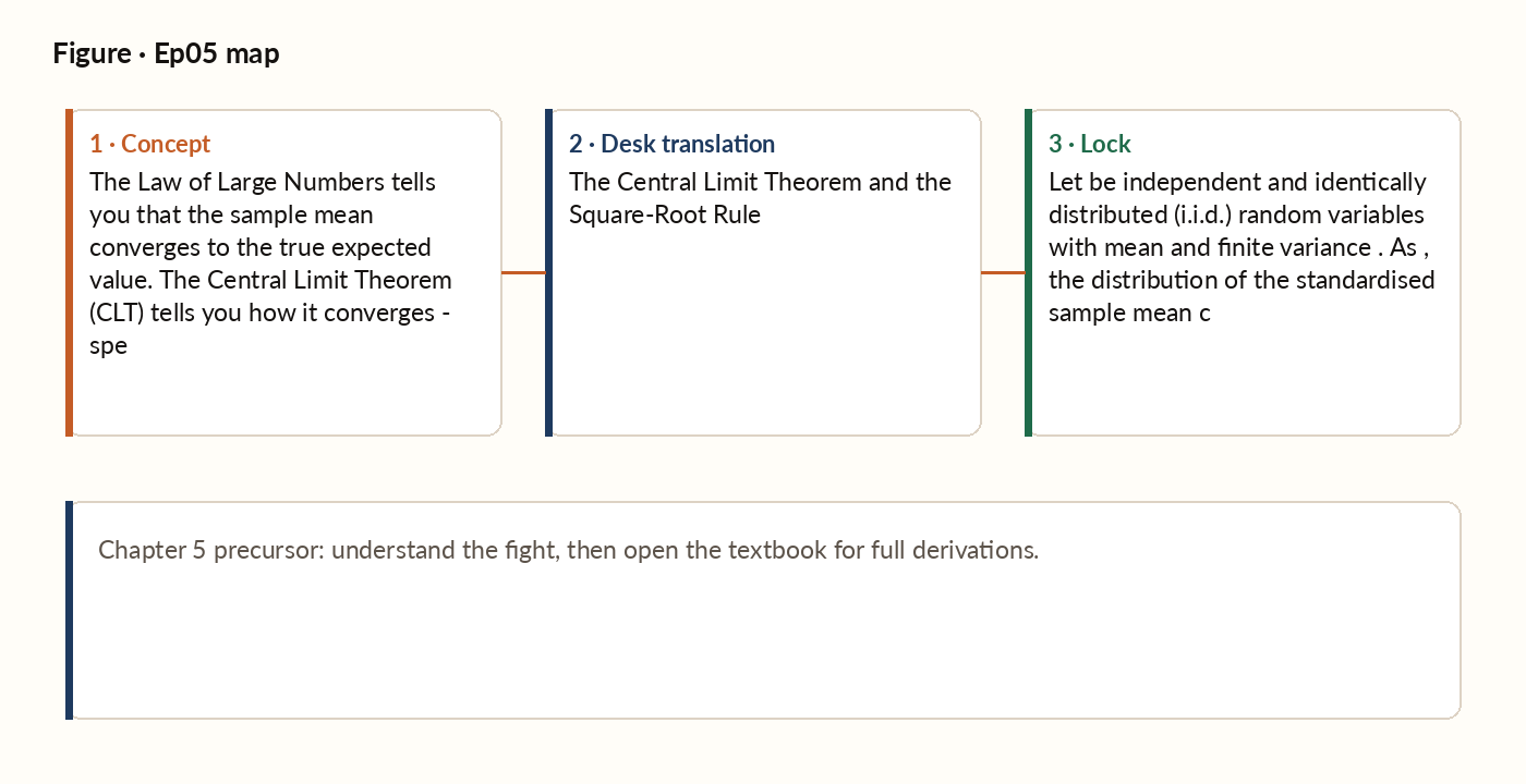
Figure 1. Concept map for this episode: fight, desk translation, what to lock.
The statement
Two things are extraordinary about this. First, the underlying distribution of any single trade can be almost anything - a coin flip, a skewed R-multiple, the daily return of a stock - and as long as it has finite variance, the sample mean is approximately normal once you have enough trades. That is why the normal distribution shows up everywhere in statistics: not because nature itself is normal, but because averages of nature are. Second, the approximation is good for most distributions once you have around 30 trades, and good enough for a simple win/loss bet once you have around 50.
Why this matters for trading
The CLT lets us answer questions like: "After 200 trades, my realised mean R-multiple is 0.18. The strategy was designed to deliver 0.12R. Is the discrepancy meaningful or noise?" We can frame this as: under the null hypothesis that the true edge is 0.12R, how likely is a sample mean as extreme as 0.18 from 200 trades? Working the numbers, that gap is only about 0.57 standard errors above design - nowhere close to the roughly 2 standard errors you'd want to call it meaningful. The excess is well within ordinary noise.
The square-root rule applied to capital
Here is a practical application that every trader should internalise. Suppose you have a strategy with a 0.15R edge per trade and realistic per-trade variability. You allocate a fixed amount of capital per R. As you take more trades, your expected total profit grows in proportion to the number of trades, but the noise around that profit only grows with the square root of the number of trades. That gap is what makes patience pay: after 100 trades your edge and your noise are roughly the same size; after 1,600 trades, your edge is about four times larger than the noise. The signal-to-noise ratio of cumulative profit improves with the square root of the trade count - the same square-root rule from Chapter 4, now applied to your P&L instead of your win rate.
Why "fat tails" make life harder
The CLT requires finite variance. For most well-behaved distributions, that condition is trivially met. For financial returns, it is met but the convergence is slow because the tails are fatter than normal. Daily stock returns, for instance, are well-known to have far more extreme outliers than a normal distribution would predict. A "six-sigma" event in a true normal distribution should happen roughly once in two million days. In actual equity markets, six-sigma daily moves happen several times a decade.
Worked picture
After 200 trades, a strategy designed for a 0.12R edge with typical per-trade swings shows a realised mean of 0.18R. Standardising that gap gives about 0.57 standard errors above design - nowhere near the roughly 2 standard errors needed for 95% significance. The CLT converts "looks good lately" into a number you can cross-examine.
What breaks in production
The CLT tells you the distribution of sample means drawn from your population. It does NOT tell you the distribution of future single trades. If your sample mean is 0.15R with a standard error of 0.05, you can say the true edge is probably between 0.05R and 0.25R. You cannot say that the next single trade will land somewhere in that range - single trade outcomes are governed by the much wider per-trade variability, not the narrow uncertainty band on the average. Confusing the distribution of the mean with the distribution of the next observation is one of the most common errors in applied statistics. The mean's uncertainty band tightens as you add trades; the next single trade's range of outcomes does not tighten at all.
Central Limit Theorem
Take many independent trades from the same underlying distribution, with a true mean and finite variance. As the number of trades grows, the distribution of the standardised sample mean converges to the familiar bell-shaped normal distribution - regardless of what the underlying per-trade distribution looked like.