The biggest risk to a stationary-feature trading model is regime change: the underlying data-generating process shifts, and the feature that predicted returns in regime A no longer predicts in regime B. A momentum strategy works wonderfully in trending years and fails in choppy ones. A mean-reversion strategy works in choppy years and gets shredded in trends. Detecting regime shifts in real time is one of the hardest and most important problems in quantitative finance. The Hidden Markov Model (HMM) is the standard mathematical framework for this problem. Originally developed in the 1960s for speech recognition by Leonard Baum and colleagues, the HMM provides a principled way to infer an unobservable system state from a sequence of observable outputs. Applied to trading, it lets us estimate the probability that the market is currently in a "calm," "neutral," or "stressed" regime - without ever needing the regime to be directly labelled. You can see the outputs (daily returns, volatility, breadth). You cannot see the regime. The HMM is a recipe for working out which regime the market is in given everything you've observed so far, using the rule that regimes tend to persist for a while before switching - essentially Bayesian reasoning across time, where each new observation updates your belief about the current regime, and today's belief carries forward as tomorrow's starting point.
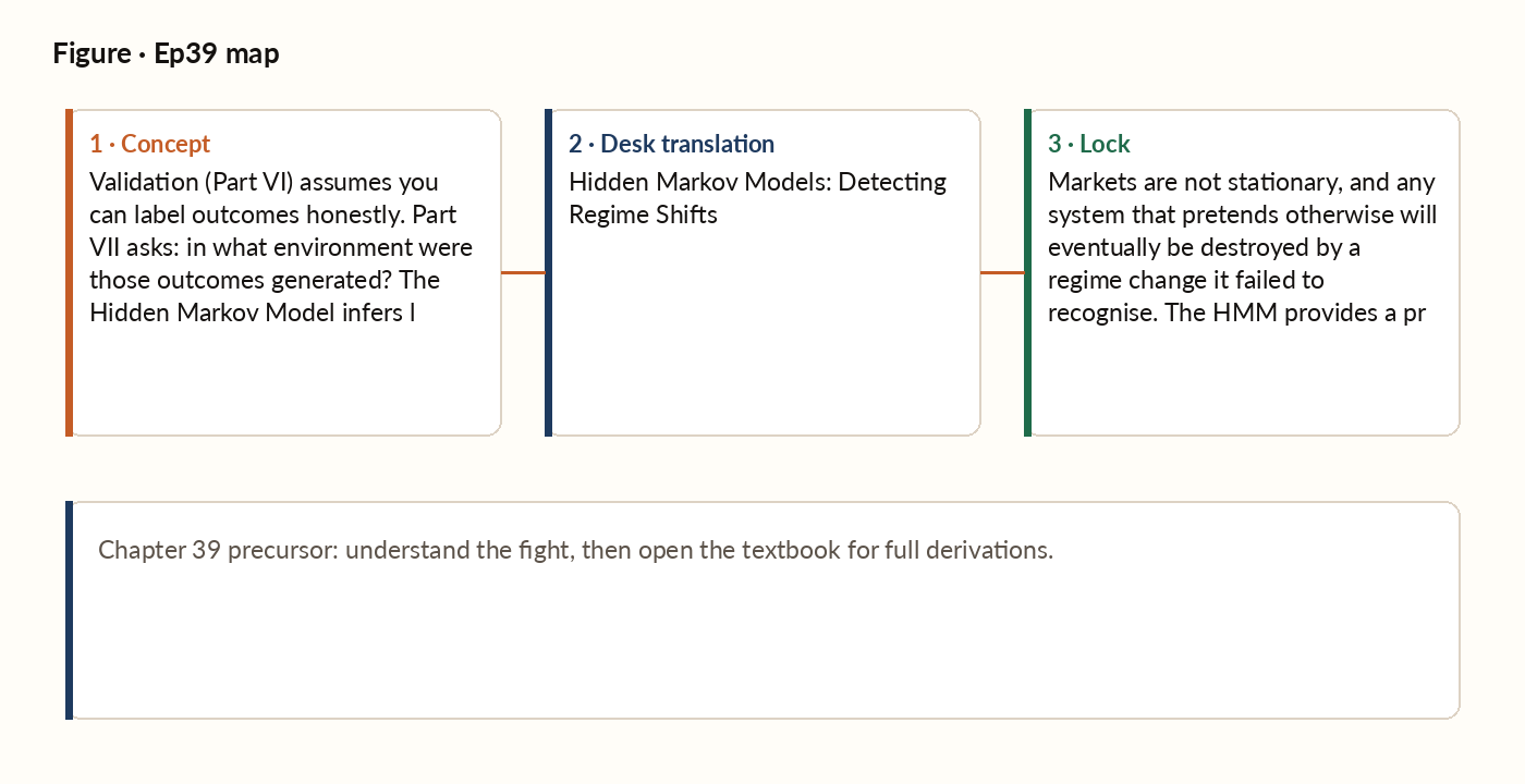
Figure 1. Concept map for this episode: fight, desk translation, what to lock.
The HMM formulation
An HMM is built from four ingredients. A state space: the finite set of possible hidden regimes (say, calm/neutral/stressed). A transition matrix: the probability of moving from each regime to each other regime over one period - each regime's row of odds always sums to 100%. Emission distributions: what the observed data (returns, volatility) typically looks like while the market sits in a given regime - often modelled as a simple bell-curve distribution per regime. And an initial distribution: the prior belief about which regime the system starts in before any data arrives. The model assumes the hidden regime evolves as a Markov chain (tomorrow's regime depends only on today's, not on the whole history) and that what you observe on a given day depends only on the current regime, not on past regimes or past observations. These are simplifications - real markets have memory beyond one period - but they are usually good enough for practical regime detection.
The three classical problems
Given a sequence of observations from an HMM, three classic problems arise. Evaluation: how likely is this observed sequence under the model at all? Solved by the forward algorithm, a dynamic-programming recursion. Decoding: what is the single most likely sequence of hidden regimes that produced these observations? Solved by the Viterbi algorithm. Learning: what model parameters (the transition probabilities, the per-regime distributions) best fit the data in the first place? Solved by the Baum-Welch algorithm. For trading, the most useful of these is a close cousin called filtering: at each moment, what is the probability the market is in each regime right now, given everything observed so far? The forward algorithm computes this as a byproduct, and it updates naturally as each new day's data arrives.
Mapping regime labels to action across horizons
The HMM outputs a belief over hidden states - but regime tags are not buy/sell commands. The same "defensive" label tightens swing entries, modulates intraday TWAP, and shifts options toward credit structures. The detector is shared; the mapping is per sleeve. Regime labels are not universal commands. The same "build" or "defensive" tag means three different things once the horizon and the instrument change.
A two-state market regime HMM
The simplest useful HMM for trading has two states: "calm" and "stressed." A typical transition matrix: the calm state persists with probability 0.95 (transitions to stressed with probability 0.05). The stressed state persists with probability 0.80 (transitions back to calm with probability 0.20). The asymmetry - stressed periods exit more readily than calm periods drag on - matches how markets actually behave: panics resolve faster than they build.
Definition
A stochastic process has the Markov property if, given the present state, the future is independent of the past. In words: the current state is a sufficient statistic for predicting the next state. The system has "no memory" of how it got to the current state - only of where it is now.
Worked picture
Suppose the past 30 days have been calm: index returns averaging +10 bps with vol 1%. The HMM's belief: 95% probability calm. Day 31: index returns -3% on no news. The emission likelihood under "calm" is very low (a 3-sigma event); under "stressed" it is moderate. After the forward update, the posterior belief shifts to perhaps 60% calm, 40% stressed. Day 32: another -2% day. Emission likelihood again favours stressed. The posterior now: 25% calm, 75% stressed. The system crosses the 70%-stressed threshold and reduces risk for tomorrow. Day 33: market rebounds +1%. Emission likelihood is roughly equal under both regimes. The posterior drifts slightly toward calm but stays in stressed territory: 30% calm, 70% stressed. The transition matrix's persistence bias - each regime tending to stick with itself - resists fast switching. This is the HMM's value: it does not panic-switch on a single bad day, but it adapts as evidence accumulates. The smoothing is principled, derived from the Markov-chain prior on regime persistence.
What breaks in production
A four-state or six-state HMM can fit the historical data better than a two-state one - it has more parameters to wiggle. But the additional states often have no real-world interpretation and produce regime classifications that are unstable in production. The principle: prefer the simplest model that captures the qualitatively important regimes. Two or three states (calm, neutral, stressed) usually suffices. Resist the temptation to add states just because the likelihood improves; ask whether each state has a clear, interpretable, persistent identity. If you cannot explain the state in words to a non-quant, you should not be using it for trading.
A narrower cousin: blending a thin recent read with a long history
Full HMM filtering earns its complexity when the hidden thing genuinely evolves over time. But a smaller version of the same problem shows up constantly: you need one number today (say, this week's volatility) and you have two honest, conflicting estimates of it - a long historical average that barely moves but is stale, and a short recent-window estimate that is current but noisy. Precision-weighted blending answers this by weighting each estimate by its own precision (one over its variance): the noisier estimate gets discounted, the more reliable one dominates, and the two combine into a single minimum-variance estimate instead of a coin-flip choice between "trust history" or "trust this week." This is exactly the update step of a Kalman filter run with no dynamics - a single hidden number held still rather than allowed to drift - which is why it is sometimes called the static Kalman update. The forward-algorithm belief update above is the same fusion idea one level up: instead of blending two point estimates, it blends a prior belief over regimes with today's new evidence.
Key idea
Markets are not stationary, and any system that pretends otherwise will eventually be destroyed by a regime change it failed to recognise. The HMM provides a principled framework for detecting regime shifts in real time, but the lightweight rules-based "HMM-lite" alternative captures most of the value with a fraction of the complexity. Either way, a regime-aware system that reduces risk in stressed conditions outperforms a regime-blind one over any meaningful horizon. And whenever the question shrinks from "what regime is this" to "how much should I trust a thin recent sample," precision-weighted blending - the static Kalman update - is the honest way to let sample size, not opinion, decide.