The IC tells you whether a feature is correlated with returns. Linear regression tells you something more: exactly how much return per unit of feature, with a complete machinery of statistical tests for significance. This chapter develops simple and multiple regression, and shows how each component of the regression output answers a specific question that a feature researcher must ask. A simple linear regression models the realised return of an asset as a straight-line function of a single feature, plus noise.
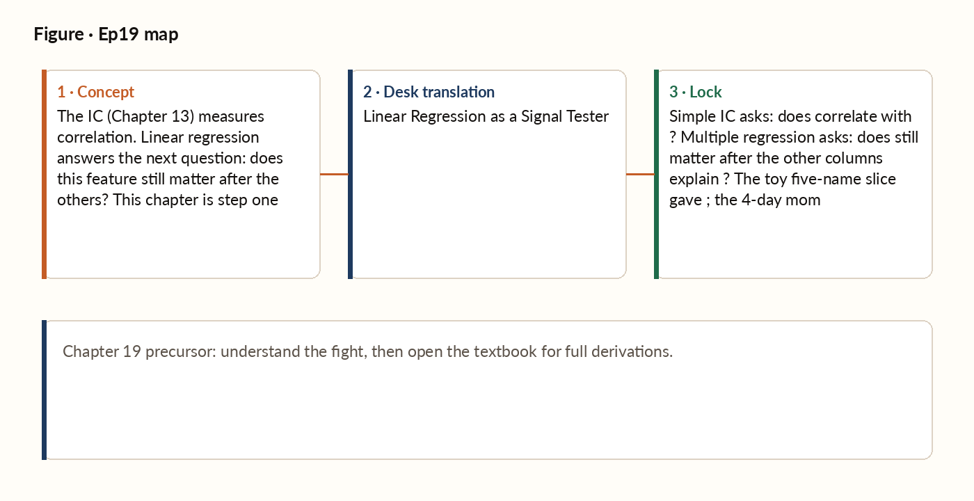
Figure 1. Concept map for this episode: fight, desk translation, what to lock.
Simple linear regression
A simple linear regression models the realised return of an asset as a straight line through a single feature, plus noise: an intercept, a slope coefficient that captures how much return moves per unit of feature, and an error term that's assumed to average out to zero. Fitting the line just means finding the intercept and slope that best explain the observed pairs of feature and return.
Connection to the IC
The simple regression slope and the IC are closely related. If both the feature and the return are standardised to the same scale, the slope equals the Pearson correlation, which is the IC. More generally, the slope is the correlation rescaled by the ratio of how spread out the return is versus the feature. So the slope and the IC are scaled versions of each other; running a regression and computing the t-statistic of the slope is equivalent to computing the IC and its t-statistic, with the same conclusion about significance.
Multiple regression
Multiple linear regression generalises the simple version to many features at once: instead of one slope, you get a whole vector of coefficients, one per feature, each estimated jointly so that every feature's effect is measured after accounting for all the others.
The crucial concept of incremental contribution
This is where multiple regression earns its place in feature research. Suppose you already have a panel of 10 features. You want to test whether a new candidate feature adds value on top of the existing 10. The right test is not the simple IC of the new feature with returns. That number tells you the total correlation, which includes the part already captured by the existing 10 features. The right test is the partial coefficient in a multiple regression that includes all 11 features. If that partial coefficient is significantly different from zero, the new feature contributes real incremental information beyond what was already there.
Worked picture
Cross-section at one date. Five stocks, each with a 5-day return and a next-week return: roughly +4.0% and +2.1%; +2.0% and +1.0%; 0.0% and −0.3%; −2.0% and −0.8%; −4.0% and −1.9%. Fitting a line through these five points gives a slope of about 0.49 - each extra 1% of 5-day momentum associates with +0.49% next-week return in this toy slice. With only five names the t-statistic is noise; the arithmetic is the point.
What breaks in production
When two features in your panel are highly correlated, their individual coefficients become unstable - small changes in the data can produce large changes in the estimated coefficients, often with offsetting signs. The standard errors balloon, and the individual t-statistics drop below significance even though the joint contribution of the two features is real. The diagnostic is the variance inflation factor (VIF): for each feature, regress it on all the other features, and the fraction of its variance explained by that auxiliary regression translates directly into a VIF score. A VIF above 5 indicates problematic multicollinearity; above 10 is severe. The fix is residualisation - Chapter 20 develops the technique that turns multicollinear features into incremental contributors. Residualisation is the central technique of professional alpha combination.
Chapter 19 — the picture closes
Simple IC asks: does the feature correlate with returns? Multiple regression asks: does the feature still matter after the other columns already explain returns? The toy five-name slice gave a real, meaningful slope; a redundant feature built from ones already in the panel gives a slope of essentially zero - same machinery, opposite verdicts. Partial coefficient → residual → combination weight is one chain. Chapter 20 strips overlap; Chapter 21 sets weights; Chapter 22 turns the composite into a probability. You met regression as a tester; the rest of Part IV treats it as the spine of honest combination.