This chapter introduces Bayes' rule from scratch, applies it to the most common trading question ("what is my true win rate, given that I've observed some number of wins out of some number of trades?"), and develops the machinery that underpins the Bayesian Kelly criterion in Chapter 9. Bayes' rule says: the probability of a hypothesis given the data you observed is proportional to how likely that data would be if the hypothesis were true, weighted by how likely you thought the hypothesis was before you saw any data at all.
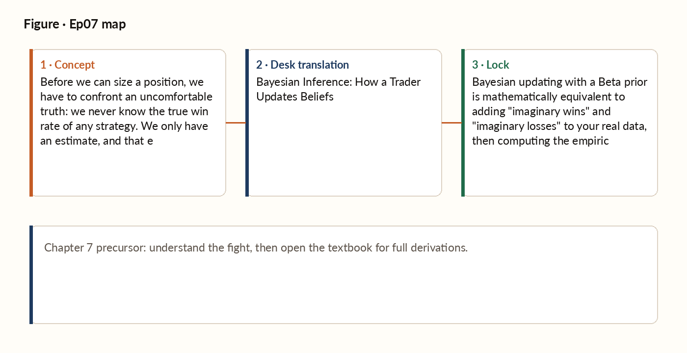
Figure 1. Concept map for this episode: fight, desk translation, what to lock.
Bayes' rule
Suppose we want to know the probability of some hypothesis (e.g., "this strategy has a 55% true win rate") given some observed data (e.g., "the strategy won 11 of its last 20 trades"). Bayes' rule, derived from the definition of conditional probability, tells you exactly how to combine your prior belief with the new evidence into an updated, honest belief, no discretionary judgement, the arithmetic does it for you.
The beta-binomial machinery
For trading applications, we almost always model the win/loss outcomes as a coin-flip-style bet with some unknown true win rate. The natural Bayesian framework asks: what is your updated belief about that win rate after seeing a certain number of wins in a certain number of trials? The right family of prior belief to use here is called the Beta distribution, chosen because it combines cleanly with binomial win/loss data and keeps the math tractable.
The crucial update rule
Here is the magic. If you start with a Beta-shaped prior belief and then observe some wins and losses, the posterior belief is again Beta-shaped. You simply add the number of wins to one of the prior's parameters and the number of losses to the other. That is the entire Bayesian update for a win/loss model. The posterior is again Beta, which means you can update it again with new data and stay in the same family indefinitely.
What this means in practice
The posterior mean win rate, after observing new wins and losses on top of a Beta prior, comes out to a weighted blend of the prior and the new data. This formula has a beautiful interpretation. The prior's two parameters act as pseudo-counts of imaginary prior wins and losses. Their total measures how much weight your prior carries. A prior worth 10 imaginary trades is easily swamped by 100 real trades, while a prior worth 1,000 imaginary trades barely moves even after 100 real ones.
Definition
A prior distribution that, when combined with the likelihood via Bayes' rule, produces a posterior of the same family. The Beta distribution is conjugate to the binomial likelihood: a Beta prior plus a binomial observation yields a Beta posterior.
Worked picture
You start with a prior that says, "I think this strategy wins about 55% of the time, but I am only moderately confident." You encode this as a prior worth 20 imaginary trades, with a mean of 0.55. After 30 real trades, you have observed 14 wins and 16 losses. Blending the two gives a posterior mean of 0.50. Notice what happened. The realised win rate was about 0.467, well below the prior mean of 0.55. But the posterior is 0.50, not 0.467. The prior pulled the estimate up because the prior was non-trivial (20 imaginary trades). The data pulled it down. The Bayesian posterior is the rational compromise. If you had used a flat, uninformative prior instead (representing complete ignorance), the posterior would land at about 0.469, almost identical to the raw data. The strength of the prior is exactly what controls how much the data moves the estimate.
What breaks in production
A common mistake in early-stage trading systems is sizing positions using the empirical win rate computed from the system's first few weeks of trading. With 20-30 trades, the empirical win rate is essentially noise. Sizing on it amplifies the noise into position-size variations that have nothing to do with the underlying edge. The professional alternative: use the posterior mean from a Bayesian update, with a meaningful prior (typically derived from the strategy's backtest or from a similar-strategy baseline). This shrinks early estimates toward sensible defaults and prevents catastrophic over- or under-sizing while the system collects evidence. The exact mechanics (how the posterior mean and posterior variance feed into the Kelly fraction) are developed in Chapter 9 (Bayesian Kelly). Beyond the posterior mean, the Bayesian framework also gives you the posterior's own uncertainty, which tells you how confident your belief actually is, and that uncertainty shrinks with more data, following the same square-root rule as everything else in this book.
The pseudo-count interpretation
Bayesian updating with a Beta prior is mathematically equivalent to adding "imaginary wins" and "imaginary losses" to your real data, then computing the empirical win rate. The strength of the prior is measured by the total imaginary trade count it represents. This makes the meaning of a "weak" or "strong" prior precise.