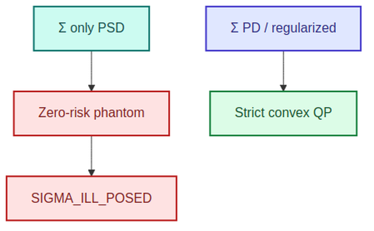
Simple claim: a merely positive-semidefinite Σ has zero-variance directions; an optimiser will monetise estimation error along them and print a free lunch. The trench is the phantom arbitrage and the definite-ness gate.
The optimiser output that should frighten you is not a large number. It is a small one.
Somebody runs the allocation job, and the minimum-variance line of the report comes back at 0.02 percent. Or 0.00 percent. The weights beside it are large and offsetting, several hundred percent gross, long one thing and short two others. Nobody built that portfolio on purpose. The solver was asked to minimise variance and it did, extremely well, and the number it produced is not a portfolio property at all. It is a property of the matrix you handed it.
What "positive semidefinite" actually permits
Problem in one line: a covariance that is only positive semidefinite has zero-variance directions. Optimisers find them and monetise estimation error as free lunch.
Every covariance matrix is real, symmetric and positive semidefinite. That is a theorem, not a modelling choice: variance cannot be negative, so the quadratic form cannot be negative. The word doing quiet work is semi.
Positive definite means every nonzero portfolio has strictly positive variance. Positive semidefinite allows equality, there can be a direction in weight space whose variance is exactly zero. If your estimate is positive definite, the mean-variance problem is strictly convex, the solution is unique, and the phrase "the optimal portfolio" is meaningful. If it is only semidefinite, both of those go away at once.
Here is the smallest concrete version. Three assets. The first has 15 percent volatility, the second 25 percent, correlation 0.20 between them. The third is defined, exactly, as an equal-weight combination of the first two, a fund holding both, or an index, or the same exposure booked through a different instrument. Build the covariance matrix from that relationship and it has an exact null direction: hold half of the first and half of the second against one unit short of the third, and the variance of that combination is zero. Not small. Zero, by construction, because the position holds nothing.
That direction is free to add to any portfolio without changing its variance. Which means it is free to add to any portfolio without changing its reported risk, and if it changes expected return at all, the optimiser will use it without limit.
Why the estimation error turns it into a phantom lunch
The relationship says the third asset's expected return must be the average of the first two, which is 10 percent. But expected returns are estimated, and estimation is noisy, so the input vector says 8, 12 and 11 percent. The third entry is 100 basis points off, an ordinary, unremarkable estimation error on a mean.
Now the null direction has a price. Moving along it changes expected return by 1 percent per unit and changes variance by nothing. Start from equal weights: 15.81 percent volatility, 10.33 percent expected return. One unit along that direction gives 11.33 percent expected return at 15.81 percent volatility, weights now minus 16.7, minus 16.7 and 133.3 percent. Keep going and the return keeps climbing while volatility never moves. The only thing that stops the optimiser is a constraint with nothing to do with risk: under a 300 percent gross cap it halts at minus 50, minus 50 and 200 percent, having bought 167 basis points of expected return at literally zero additional variance.
Every number in the report is arithmetically correct: volatility unchanged, return higher, Sharpe improved. What actually happened is that 100 basis points of noise in one expected-return estimate got levered against a rank deficiency until it hit the only binding constraint in the problem. A portfolio sitting precisely on a use cap with an unchanged risk number is the signature.
Why it feels like elegant mathematics
Because the closed-form solution is beautiful and it does not warn you. With shorts allowed and only a budget and return row, the optimum is the inverse covariance applied to a combination of the ones vector and the expected-return vector, with multipliers from a small Gram system in the usual moment quantities. It fits on a slide, and it is the version most people carry in their heads.
It also requires the matrix to be invertible. When the matrix is singular the inverse does not exist and the Gram system's determinant vanishes, an error in exact arithmetic, and something worse in floating point. The smallest eigenvalue comes out around ten to the minus eighteen rather than zero, the linear solve succeeds, and out comes a confident weight vector determined largely by rounding. Reported variance prints as 0.00 percent. No exception, no warning, and no field in the report where the condition number would have appeared.
And on real data, rank deficiency is not an exotic case, it is the default. A sample covariance matrix estimated from sixty monthly observations across eighty names has rank at most fifty-nine. That guarantees at least twenty-one exactly-zero-variance directions before anyone does anything wrong. You do not need a redundant asset. You just need more names than observations, which describes most books.
How this shows up in production
- The suspiciously tiny risk number. Minimum variance reports near zero with hundreds of percent of offsetting gross. Someone calls it a relative-value opportunity. It is a null space with a use cap.
- Silent pseudo-inverse repair. A library detects the singularity and quietly regularises, a ridge, a pseudo-inverse, a nudge to the diagonal. The job succeeds, the answer depends entirely on the size of that nudge, and the nudge is on no card. Two libraries with different defaults give different portfolios and both call themselves optimal.
- Duplicate exposures through different instruments. The same underlying held directly, through a fund, and through a swap. Nobody added a redundant asset on purpose; the position taxonomy did it, and the dependence is invisible in a position report and structural in the covariance matrix.
- "The optimal portfolio" as a claim. Without strict convexity the solution set can be a line or a flat region, so a report naming one point as the optimum has silently picked a member of a set, and which member depends on solver internals.
- Degenerate geometry in the certificate. Redundancy can cost the active constraint gradients their independence, so the constraint qualification fails and the multipliers stop meaning anything, the inconclusive the proposal audit exists to return, if anyone checks.
A walkthrough on CEH-001
| Symptom | Reading | Gate |
|---|---|---|
| Min-var line reports σ≈0.00–0.02% with huge gross | Null direction of Σ exploited | refuse / regularise |
| Long one name, short two others, offsetting hundreds of % | Phantom arb from estimated μ along null of Σ | SIGMA_SINGULAR or rank fail |
| CEH dual marks “hedged” to zero vol in optim | Frame gap laundered into null portfolio | joint Σ must be PD enough for rights |
| Eigenvalue floor / shrinkage not carded | Silent regularisation differs research vs serve | hash regularisation recipe |
The structured book, marked near 1.50 under the spread frame and near 2.10 under the curve frame.
The book's covariance matrix is built from mark histories, and the marks are constructions, every one of them a function of the same bootstrapped curve and the same convention set. Several cousins are, to a very good approximation, linear combinations of the others: same curve exposure, same convention sensitivity, different tenor labels. That approximation is exactly what a rank-deficient matrix looks like before floating point rounds it off.
So the allocation job finds the near-null directions and loads them. The output is a hedge-heavy construction with a reported volatility below anything the desk has ever experienced on this book, several hundred percent gross, and an expected return improved by a bit under two percent. It is presented as the risk-reducing trade. It is a levered bet on 100 basis points of mean-estimation error inside a linear dependence created by the marking machinery.
Then the argument comes back to the marks, and this is the part I find most instructive. The construction only makes sense if the two frames are close, because it assumes the cousins substitute for each other cleanly. So the trade needs the gap to be small, and the number that makes it small is 1.80. A portfolio built out of a null space is now generating pressure to invent a mark. The optimiser did not ask for 1.80. It made 1.80 convenient, which in an organisation under deadline is nearly the same thing.
What stacks quietly assume
They assume any covariance estimate is invertible, that a successful linear solve means a well-posed problem, that the minimum-variance number is a risk statement rather than a rank statement, that there is one optimum, and that regularisation defaults are neutral. They assume redundancy would be obvious, when it arrives through instrument taxonomy and short samples. And they assume a small risk number is good news, when a small risk number with large offsetting weights is the most reliable tell that the model has stopped describing the world.
What a solution must do
Problem: PSD (not PD) Σ plus noisy μ creates zero-risk directions that optimisers treat as free expected return. Solution: enforce positive-definiteness / eigenvalue floors as card fields, refuse or regularise with a hashed recipe, never promote zero-vol books without an economic story that survives a risk-free rate check (see S2-09).
What to lock
- Minimum eigenvalue (or condition number) of Σ is a card field; fail then refuse or regularise under named recipe.
- Regularisation / shrinkage parameters are hashed with the covariance recipe (S2-06).
- Portfolios with near-zero model vol and large gross escalate as
PHANTOM_ARBcandidates. - CEH joint risk under dual frames cannot “optimise away” the 0.60 frame gap into a null direction.
- Research and production must share the same PD gate; silent eigenvalue clipping is a silent frame.
Clearance coupling: optimisers do not get to invent riskless excess return from estimation geometry. Next: perfect correlation limit (S2-09).