Suppose at the start of each period, you rank every stock in your universe by some feature - a value score, a momentum score, whatever you like. Over the next period, each of those stocks earns a real return. The Information Coefficient for that period is just the correlation between the feature ranking and the realised returns: a single number between -1 and +1. A positive IC means the feature worked - stocks it ranked highly went on to do well. A negative IC means it worked backwards. An IC near zero means the feature told you nothing that period.
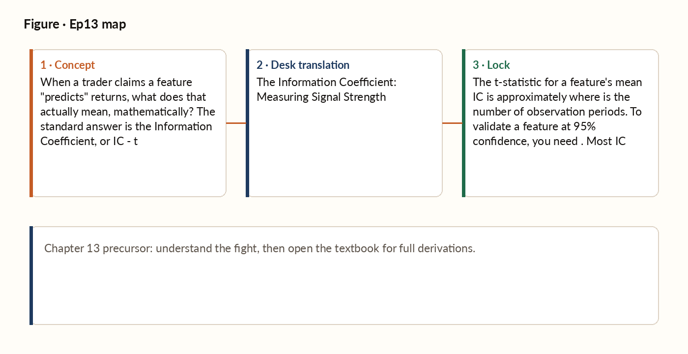
Figure 1. Concept map for this episode: fight, desk translation, what to lock.
The definition
Suppose at the start of each period, you rank every stock in your universe by some feature. Over the next period, each stock earns a real return. The Information Coefficient for that period is the correlation between the feature ranking and the realised returns - a single number between -1 and +1. A positive IC means the feature positively predicts returns at this period: stocks with high feature values tended to deliver high returns. A negative IC means the feature negatively predicts: high feature values predicted low returns.
Why IC is usually tiny
Here is the uncomfortable fact about IC: even excellent features have small ICs. A feature with a mean IC of 0.05 is considered outstanding. A feature with a mean IC of 0.10 is industry-leading. ICs above 0.15 - sustained, out of sample - are essentially nonexistent in liquid markets. This is not a failure of the measurement; it is a measurement of how hard the underlying problem is. Markets are dominated by noise. The signal-to-noise ratio of any feature, even a very good one, is small in absolute terms. The job of a quantitative researcher is to find as many small, genuine edges as possible and combine them - no single feature is expected to carry a strategy on its own.
The relationship between IC and t-statistic
If a feature's mean IC across many periods is small, how many periods do you need to observe before that estimate is statistically distinguishable from zero? The answer connects IC directly to the t-statistic and to Chapter 5's square-root rule: the more periods you observe, the more the noise in your IC estimate averages out, and the estimate's standard error shrinks roughly with the square root of the sample size.
IC variants
Several variants of IC appear in the literature and in practice. Pearson IC is the standard linear correlation defined above. Sensitive to outliers; assumes a linear relationship. Spearman IC replaces the raw feature values and raw returns with their ranks within each period (1st, 2nd, 3rd, ...) before computing the same correlation. Because only the ordering matters, one extreme outlier can't drag the number around the way it can with Pearson, and Spearman doesn't require the relationship to be a straight line, only that a higher feature value tends to go with a higher return, however that curve bends.
Definition
The (cross-sectional) Pearson correlation between a feature value and the subsequent realised return, computed across all assets observed at the same time. Often summarised as the mean IC across many periods, with a standard error.
Worked picture
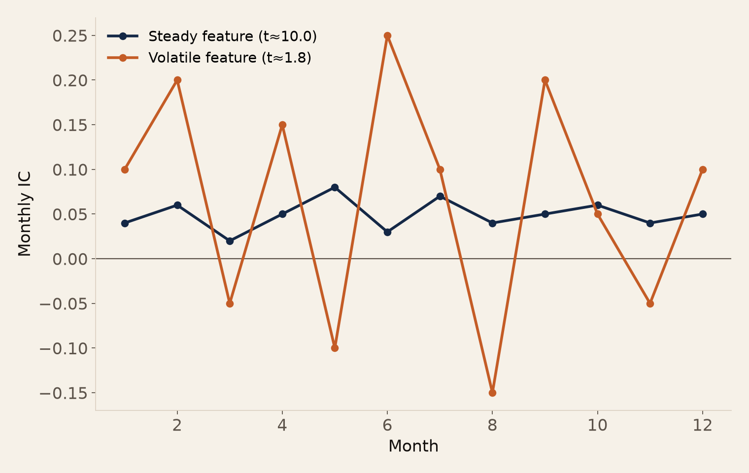
Over 12 months, you compute the daily Spearman IC of a feature against next-day returns. The 12 monthly mean ICs are: 0.04, 0.06, 0.02, 0.05, 0.08, 0.03, 0.07, 0.04, 0.05, 0.06, 0.04, 0.05. The 12-month mean IC is about 0.05. The monthly ICs barely move around that average (a standard deviation of roughly 0.017), so the estimate is precise: the resulting t-statistic works out to about 10 - very strongly significant. This is what an excellent feature looks like in IC space. The mean is small, but the consistency (small swings from month to month) gives high confidence that the feature is genuinely predictive. By contrast, suppose the monthly ICs were: 0.10, 0.20, -0.05, 0.15, -0.10, 0.25, 0.10, -0.15, 0.20, 0.05, -0.05, 0.10. The mean is also about 0.07, similar to before. But this time the months swing wildly (a standard deviation of 0.13), and that noise drags the t-statistic down to about 1.8 - not significant at the 95% level. Despite a higher mean IC, the feature is actually less trustworthy because of the volatility. Consistency beats peak magnitude in IC analysis.
Figure. The two 12-month IC series above, plotted month by month — same order-of-magnitude mean, opposite statistical significance (t≈10.0 vs. t≈1.8).
What breaks in production
Computing the IC of a feature on the same data you used to design the feature gives an inflated estimate. If you derived a feature by searching across many candidates and keeping the one with the highest in-sample IC, you have data-mined the feature, and the in-sample IC dramatically overstates the out-of-sample IC. The next chapter develops this trap formally as the multiple testing problem. For now, the rule: never report the IC of a feature on the same data you used to design it. Always reserve a holdout sample, and report the holdout IC as the honest estimate.
The IC-to-t-stat shortcut
The t-statistic for a feature's mean IC grows with the square root of how many periods you've observed - so a feature with a real but small IC still needs a long track record before you can trust it. Most ICs are too small to validate in any reasonable timeframe - which is why feature research requires long histories and many features, combined via the Fundamental Law of Active Management (Chapter 17).