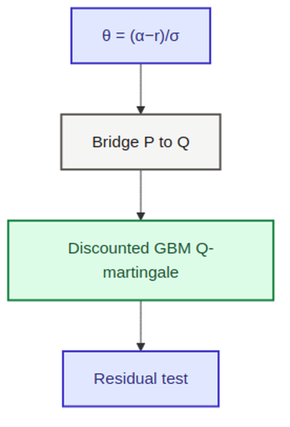
Simple claim: θ = (α − r)/σ is the bridge that lets a forecast and a price share one model without contaminating each other. The trench is price of risk on the card before either story spends.
The problem we left open
Problem in one line: without θ = (α−r)/σ on the card, forecasts and prices contaminate each other and silent Girsanov overlays stay loadable.
Last time I argued that a drift overlay is the hardest failure in the stack to catch, and the argument was uncomfortable: Girsanov leaves quadratic variation alone, so the volatility check passes under either measure, and estimating a five-point drift gap from a 20-vol series needs decades of history you do not have. Monitoring cannot rescue you. The measure has to be declared at construction.
Which raises the obvious objection. If a path set must be tagged with its measure, and pricing must refuse the physical one, what connects them? The desk needs both: a view on where the stock is going, and a price that reflects what a hedge costs. Two dynamics for one instrument sounds like two models, two calibrations, and two opportunities to mix them up.
Three production headaches:
- Forecasting and pricing maintained as separate models of the same asset, drifting apart in volatility, calibration date, even sign conventions.
- No artifact recording the relationship between them, so an auditor cannot check consistency and an engineer cannot detect a swap.
- Hedging residual attributed to "model error," because no stated quantity exists whose misstatement would produce exactly that residual.
So the question for this post is simple. If that is the failure mode, what does a real AI solution look like?
The solution, as one stack
The core idea: the two worlds are not two models. They are one model and one number. Write the asset once under the physical measure, and the risk-neutral dynamics follow from a single scalar, the market price of risk, that you compute, post, and audit. Five moves, one stack.
1. Write the physical dynamics explicitly, and only once. Geometric Brownian motion: dS = αS dt + σS dW, with α the mean return and σ the volatility, under P. Itô gives the explicit solution, an exponential of a normal, which is why S stays strictly positive. This is the only place α and σ get calibrated. Everything else derives.
2. Name the discount object. The bank account grows deterministically at the short rate; its reciprocal, D_t = exp(−∫₀ᵗ r_s ds), is the stochastic discount factor. Pricing is a statement about the discounted asset, never the raw one, and keeping D explicit prevents the constant-rate shortcut from hiding a rate-convention mismatch with the instrument's own cashflow contract.
3. Solve for θ and post it as a required field. There is exactly one tilt that turns the discounted stock into a martingale:
θ = (α − r)/σ.
The market price of risk: excess return per unit of volatility. Compute it, write it on the measure card, and make it mandatory on any artifact claiming to be risk-neutral. This is the number the last post said was missing, and it makes the two measures auditable against each other, given any two of α, r, θ, the third is determined, so an inconsistency in the triple is a check a machine can run.
4. Bind consumers to exactly one drift. Under Q the dynamics become dS = rS dt + σS dW̃. Read that plainly: under the pricing measure, the stock and the bank account have the same expected return. That is not a claim about the world; it is the definition of the measure in which hedging costs are computable. So forecasting binds the α-dynamics, pricing binds the r-dynamics, and no process holds both. A service that can reach either drift will eventually reach the wrong one: MIXED_DYNAMICS is a structural refuse, enforced by what a component may import rather than by code review.
5. Close the loop with the residual test. This recovers the detection the last post seemed to rule out. You cannot see a drift error in the price path, because the drift is buried under σ. But hedging removes most of that σ, and what remains is a residual series with far less noise to hide behind, so a systematic drift error that was undetectable in the underlying becomes visible as a residual that leans one way. The residual card is therefore also the drift monitor. Declaration governs construction; the residual catches what declaration missed.
Put together: one calibrated physical model, an explicit discount factor, θ computed and posted, consumers bound to a single drift each, and a residual series that reveals errors the price path conceals. That is the measure bridge. Both worlds stay available. Neither can borrow the other's drift.
The example: CEH-001's equity leg, with θ on the card
| Price of risk card | Value |
|---|---|
| Physical α, σ | 10%, 20% |
| Short rate r | 5% |
| θ = (α−r)/σ | (0.10−0.05)/0.20 = 0.25 |
| Q drift of underlying | r = 5% (σ untouched) |
| Discrete twin Z | (0.9375, 1.25) from p=0.80, q=0.75 |
| Load rule | Pricing consumers load Q-paths only |
| Wrong load that faked mid of 1.50–2.10 | Fails at load, not at “vol looks fine” |
Same never-traded note, same leg, now in continuous time. The physical calibration gives α = 10% and σ = 20%. The short rate on the note's own as-of curve is r = 5%.
One line: θ = (0.10 − 0.05)/0.20 = 0.25.
That is the entire bridge. Under P the leg's underlying drifts at 10%. Under Q it drifts at 5%, the short rate, with σ = 20% untouched, because the tilt moves drift and never touches noise. Both facts go on one card, together with θ, the as-of clock, and the calibration window.
Check the continuity with what the tree already told us. In the discrete world the tilt was Z = (0.9375, 1.25), derived from p = 0.80 and q = 0.75, with q coming from (u, d, r) and no estimation. Here the tilt is the exponential martingale built from θ, and θ comes from (α, r, σ). Same structure at two resolutions: the unique reweighting that removes the risk premium, determined by the world card rather than chosen.
Now the operational payoff. The exposure study from the last post, the one that passed its volatility check while carrying a physical drift, becomes impossible to run silently. The path artifact has a measure field. It has θ = 0.25 or it does not. A pricing consumer must load Q-paths, and Q-paths drift at 5%. The comfortable mark that drifted toward the middle of 1.50 and 2.10 never gets produced, because the run that produced it now fails at load rather than passing at validation.
Then the residual, where the five points actually show up. Suppose someone gets θ wrong anyway, implicitly setting it to zero by pricing with the physical drift. The hedge built off those dynamics is systematically off, and the account no longer tracks the claim in an unbiased way. The residual series acquires a lean of roughly the drift gap applied to the exposure, five percent per year on the notional at risk, which on a hedged book is enormous relative to the residual's own scale. That lean is detectable in months, because after hedging there is very little volatility left for it to hide behind. The drift you could not estimate from sixteen years of price history shows up in one quarter of residuals.
Against 1.50 versus 2.10 this changes the argument. Each frame now has to publish its θ. If the spread frame and the curve frame imply different market prices of risk on the same underlying at the same as-of, that is a concrete single-number disagreement rather than two narratives about staleness. And 1.80 has no θ at all, because it is the arithmetic mean of two numbers rather than the output of any dynamics. A mark with no market price of risk behind it cannot say what world it is a price in, the objection this series started with, now with a scalar attached.
The flow in one breath
Problem: Girsanov overlays pass vol checks. Solution: put θ on the measure card as the bridge between forecast (P) and price (Q); enforce load-time measure match; residual lean after hedge signals drift contamination. Example: CEH equity leg θ=0.25; Q-paths drift at 5%.
What to lock
theta(or full density process) is a required field on any P↔Q bridge card.- Pricing path stores are labeled Q; physical scenario stores are labeled P; cross-load is refuse.
- Monitor hedged residual for drift lean at scale of (α−r) on exposure.
- CEH dual frames: each frame’s θ/r/σ recipe is hashed; no silent path to 1.80.
- Agents may propose α forecasts; harness never prices with α as Q drift without θ card.
Clearance coupling: one number lets forecast and price share a model without contamination. Next: Black–Scholes as contrast, not ticket (S2-19).